Evaluation, Measurement, and Verification (EM&V) Report: Bassett-Avocado Heights Advanced Energy Community (BAAEC) Project
Authors:
Dr. Eric D. Fournier †
Julia Skrovan †
Robert Cudd †
Other Contributors:
Spencer Mathews †
Affiliations:
† - The California Center for Sustainable Communities (CCSC) at the University of California Los Angeles (UCLA)
Date:
Nov 14, 2025
Note: No generative Artificial Intelligence (AI) software was used in the development of this report. Its contents are the original intellectual products of the listed authors and contributors.
Table of Contents
- Advanced Homes (AH) Program
- Community Solar (CS) Program
Advanced Homes (AH) Program
Background
Program Design
Eligibility
Per the requirements of the CEC’s Advanced Energy Community grant funding opportunity, as well as those of various supplemental funding sources leveraged, such as the Disadvantaged Community Single-Family Solar Homes (DAC-SASH) program, there were a number of eligibility criteria that had to be met for households to participate in the BAAEC AH program. Most substantively, these included:
- A household income requirement - commensurate with CARE/FERA program eligibility
- A geographic location requirement - participant homes must be geographically located within census tracts designated as disadvantaged communities (DACs) according to the California Office of Environmental Health Hazard Assessment’s (OEHHAs) CalEnviroScreen 4.0 screening tool.
- A set of physical site suitability requirements - participant homes must be physically suitable for the installation of associated program measures. Satisfaction of these requirements involved a series of in-person site visits to evaluate the condition of the home’s structure and electrical equipment as well as ensure that there were no unpermitted structures or major building code compliance issues.
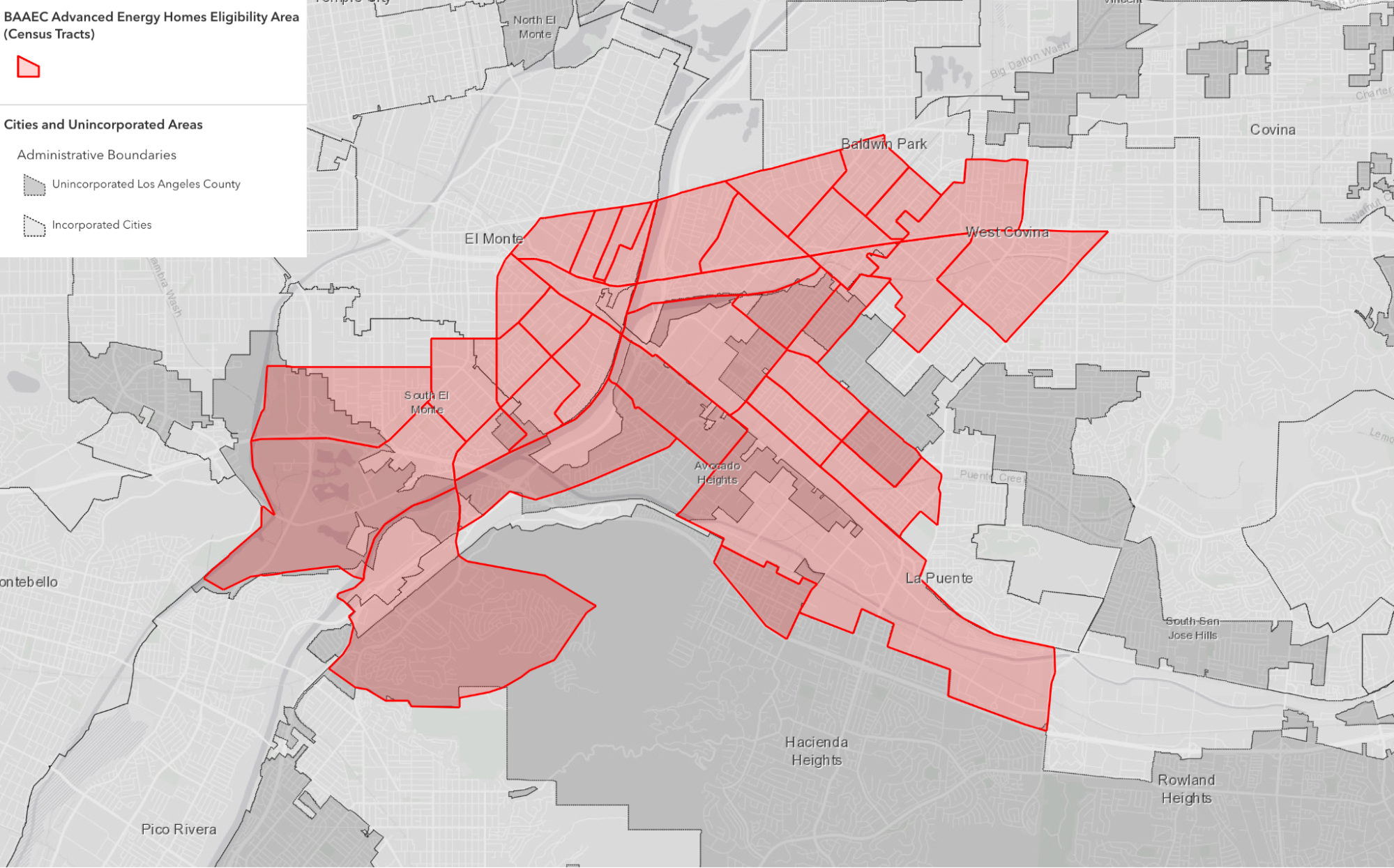
Figure 1: Map of the geographic eligibility area for participants in the Advanced Homes program (Red) relative to local municipal boundaries (Dark Gray).
The initial AH program design called for a geographic eligibility area that was restricted to a group of 4 contiguous DAC census tracts located within the Los Angeles County Unincorporated communities of Basset & Avocado Heights. However, due to challenges that were encountered in the recruitment of participants throughout the course of the project’s implementation phase it was decided, in conjunction with CEC, that this eligibility area be expanded to include 33 additional census tracts (for a total of 37) located within one mile of the original set of 4. Figure 1 shows a map of this final eligibility area relative to local municipal boundaries.
Enrollment
For community members residing within this geographic eligibility area, the choice of whether or not to participate in the BAAEC AH program was a completely voluntary decision. Recruitment of participants occurred through multiple channels including social media campaigns, local event tabling, canvasing, and other outreach methods. These recruitment outreach efforts were led by staff at a local community based partner organization called Day One who were contracted under the project, in conjunction with outreach staff at TEC and Grid Alternatives. Their work involved not only informing community members about the program’s existence, but also educating them about the various eligibility criteria, how the project was being funded, what its purpose was, as well as providing detailed information about the suite of measures on offer, how they would be installed, and what benefits they could be expected to provide.
A key tenant of the AH program’s design was that there would be zero up-front costs for all participants, regardless of the set of measures that they ultimately decided to pursue. Making this a reality however, required significant effort on behalf of the project leads at TEC to orchestrate different sources of supplemental funding to help offset the costs of any required site remediation work as well as to work with business partners on financial models capable of amortizing hardware procurement and installation costs over time. Evolutions in the design of these financial arrangements are documented in detail as part of the project’s Case Study reporting.
Measures
The AH program was advertised to potential participants as consisting of a suite of optional measures. Among these, it was initially envisioned that all participant households would minimally receive a rooftop solar photovoltaic (PV) system and accompanying battery energy storage systems (BESS). However, through the course of the project’s implementation period it became clear, in part due to the household preferences and in part due to difficulties with the project’s partnering BESS solution providers, that several AH program participants were either going to decline to receive the BESS device or that their device would not be able to be installed in time for the completion of this report.
In addition to the PV and BESS system offerings, two additional measures were available to participants. These included the installation of a new heat-pump water heater from Rheem and an induction combo stove and range from Frigidaire. Supplemental funding to support the purchase and installation of the heat pump water heaters was obtained through the TECH Clean California program, and funding for the purchase of the induction stoves was sourced through a collaboration with the Los Angeles Clean Tech Incubator (LACI). Table 1 below documents each of these available measures, including descriptions of the specific technologies used, as well as the total number of households in the AH participant cohort who opted for each. Figure 2 depicts the numbers of households within the cohort that adopted different unique combinations of these measures.
Table 1: Optional program measures available to Advanced Homes participants.
| Program Measures | Detailed Measure Description | Recipient Households |
|---|---|---|
| Rooftop Solar Photovoltaic System | A rooftop mounted solar PV system, averaging 4 kW in size. | 34 Households |
| Stationary Battery Energy Storage System (BESS) | The battery energy storage systems installed at participant homes were Tesla Powerwall 2 units which each have a rated storage capacity of 13 kWh. These are fully-integrated AC battery systems designed for residential or light commercial use which have rechargeable lithium-ion battery packs that provide energy storage for solar self-consumption, time-based control, and backup. These system installs also included a separate gateway unit which controls the battery’s connection to the grid, automatically detecting outages and providing seamless transition to backup power. It also provides energy monitoring functionality that is used by the battery for solar self-consumption, time-based control, and backup operation. | 11 Households* |
| Heat-Pump Water Heater | Rheem 50 or 65-gallon heat-pump water heaters sized according to household composition and ASHRAE standards | 20 Households |
| Induction Stove | Induction ranges (oven/ cooktop) and 240V outlets (if absent). | 9 Households |
| * The total number of battery energy storage systems installed within the period of utility consumption data availability. As of 11/5/2025 there have been 30 completed BESS installs under the AH program. Unfortunately, the remainder of these cannot be included in the analysis as they occurred after 12/31/2024. |
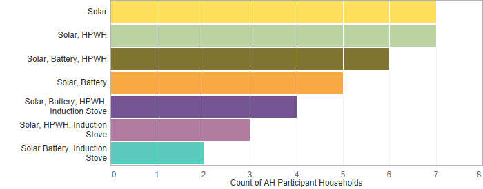
Figure 2: Distribution of the 34 AH participant households across the measure packages.
Site Remediation
As part of the AH program’s enrollment process, once a household had expressed interest in participating in the program and passed various eligibility screens, a series of site visits were performed to assess the physical condition of the home and determine the feasibility of installing various types of equipment without the need for additional site remediation work. A significant barrier that was identified by the project team, particularly for the installation of the solar PV systems, was the physical condition of the roofs of potential participant homes. A majority of the homes who were interested in and eligible for the AH program (19) were found to have roofs which were structurally unfit to support the weight and windloading associated with a roof mounted PV system. To address this issue, TEC reallocated project funding, and partnered with Grid Alternatives to contract with a third-party roofing company to do inspections and complete necessary remediation work - up-to and including full roof replacements - as necessary. In addition, Grid Alternatives took on the responsibility of performing electrical service panel upgrades for households whose existing panels did not have sufficient capacity to support the new breakers required for the rooftop PV and BES systems. Finally, a separate contractor was used to install new 240-V outlets for the HPWH and Induction stoves for recipients who opted to receive them.
Table 2: Eligible site remediation work for Advanced Homes program participants.
| Site Remediation Measures | Detailed Measure Description | Recipient Households |
|---|---|---|
| Roof Repair or Replacement | Full or partial re-roof (fascia and/or structural elements) to prepare homes for the installation and anchoring of rooftop solar PV panels. | 19 |
| Electrical Service Panel Upgrade | Replacement of existing main service panels and installation of “critical loads” sub-panels to accommodate the installation of solar, batteries, and electrified appliances. | 24 |
| 240-Volt Outlet Installation | Outlet, conduit, and wires for optional electrification measures (induction stove, HPWH, EV charger) | Every HPWH and Induction stove received a dedicated 240V new line and breaker |
| Wiring Upgrades | Miscellaneous repairs and replacement of wires, conduit, and other materials necessary for Advanced Homes retrofits |
Terms
In order to participate in the AH program, households were required to consent to a number of required conditions related to data sharing, the transfer of eligible tax-credits for installed equipment, as well as the delegation of equipment controls and/or ownership, in some cases. First among these conditions was that participants would authorize the sharing of all household energy usage and device telemetry data, where applicable, with TEC and the rest of the AH program team for the purposes of program performance evaluation.
Homeowner consent to data collection was established through a set of customer contracts and a participation form prepared by TEC. Homeowner signature of the Advanced Homes participation form, GRID Alternative’s DAC-SASH and Sunrun Third-Party Ownership forms, Swell Energy and Haven Energy’s customers service and installation contracts were necessary for the partners to collect homeowner data and share it with UCLA for the purposes of evaluation, measurement, and verification.
TEC’s homeowners participation form was necessary to authorize the use of CEC funds for and re-roofing and repair of homes prior to the installation of solar, batteries, or electric appliances. GRID’s DAC-SASH and TPO contracts collected information on home condition, household composition, income information, transferred the ownership of rooftop solar arrays and associated federal tax credits to Sunrun, and authorized the collection of telemetry data from smart inverters installed as part of Advanced Homes retrofits.
Program Implementation
Period of Performance
As documented in the project’s Case Study report, there were a number of large scale events which created challenges for the implementation of various elements of the AH program’s scope. Significantly, these factors contributed to a reduction in the number of participant households from what was originally envisioned as well as significant delays1 in the installation of specific measures relative to their originally planned timelines of execution. Both of these outcomes significantly impacted the feasibility of the UCLA team’s original technical plan for the evaluation, measurement, and verification of the AH program’s performance.
Due to the time constraints associated with the CEC’s grant funding and the need to provide reporting documentation well in advance of the project’s formal termination date, a cut-off date (12/31/2024) had to be specified regarding which AH program enrollees would be included in this EM&V analysis. The choice of this date reflected the need to provide UCLA staff with the time necessary to obtain required data from the local utilities and project partners, to analyze this data, and document as a set of reporting deliverables. Relative to this cutoff therefore, it is important to recognize both new enrollments in the AH program as well as the implementation of new measures for existing program enrollees is still ongoing and will likely continue to be so well beyond the formal completion of the CEC’s contracted project funding period.
For the purposes of this EM&V analysis therefore, the AH program participant cohort consists of a total of 34 single-family homes. The graphic on the left-hand portion of Figure 3, plots the requested program measures and their timelines of installation for each of these participant homes. Here each intervention is labeled as a colored point - the absence of which indicates refusal by a participant. The timeline itself is also colored according to the set of dates which occurred prior to (green) or following from (red) the completion of all requested measures at each participant’s home. The variable timing and duration of both these pre and post periods have important consequences for the EM&V technical methodology, as limitations on the date range (described further below) of the consumption data that was available for participant homes for the local utility providers resulted in corresponding limitations on the effective period of performance that was able to be evaluated for each home. Moreover, the mechanics of the process by which utility customer data are able to be accessed for this type of analysis is associated with significant time delays. This is an issue which shall be discussed in more detail in the subsequent methods documentation section of this report.
In an ideal analysis, data would be available for each participant for at least a full year after an intervention, with at least two years of data available in the pre-intervention period. This would mean that for every date (month and day) of the post-intervention period, there would be 2 prior corresponding days to compare it to. The sub-plot on the right hand portion of Figure 3 illustrates the extent to which such data are available for each household is denoted by a set of blue/orange colored lines. These show the range of post-intervention dates for which there are either 0 (blank), 1 (blue), or 2 (orange) corresponding pre-intervention days that could be used as a basis of comparison. As the data illustrate, only two AH participants had a full 12 month period-of-performance with multiple dates of pre-period comparison data for the majority of the year. For the rest of the participants, the effective periods of performance varied significantly both in duration and time of year (season). This unfortunate outcome has significant impacts for the interpretation for the results of various planned EM&V analyses that will be called out in subsequent portions of this report.
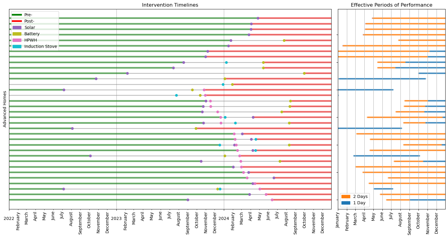
Figure 3: The sub-plot at left depicts the timelines of completed AH program interventions for each participant household. The corresponding periods of performance are plotted for each, with pre- (Green) and post- (Red) implementation dates labeled. The sub-plot to the right illustrates the effective overlap between the pre-and-post periods, in terms of the numbers of corresponding dates (1 - Blue, 2 - Orange) as a series of labeled timelines.
Methods
Data Sources
Energy Data Request Program (EDRP)
The EDRP is a CPUC mandated program which allows for academic researchers at qualifying state institutions to request energy consumption and other personally identifiable information (PII) for Investor Owned Utility customers. These data can only be used for legitimate research purposes with demonstrable rate payer benefits.
Each IOU within the state implements its own process for reviewing and responding to EDRP requests. If a request is approved, sensitive customer data may only be shared once the requesting party has agreed to a non-disclosure agreement (NDA) which stipulates, among other things, required data anonymization and aggregation procedures for the protection of customer privacy in the publication of derivative research products. Following from the agreement of this NDA, the fulfilling IOU must issue a notification to the CPUC of each request’s approval.
Once this notice has been submitted, and the corresponding waiting period served, the requesting party is able to negotiate the technical details of the request with the fulfilling IOU’s meter and customer database administrators. These IOU staffers must then have time to formulate the request into a series of database queries, export the data, and make it available via a secure file transfer portal. All of the steps in this process require extensive, manual coordination among the parties involved. As a result, the process can consume significant amounts of time. It is not uncommon for 6 or more months to elapse between the time at which a request is initially submitted and the time when the requested data is finally transferred.
Two separate EDRP data requests were submitted as part of this project, one each to Southern California Edison (SCE) and SoCal Gas, the single fuel utility service providers for the 34 total AH participant households. In addition to requesting data for these AH program participants, we additionally requested similar data for a control group of non-participant residential customers served by each utility. These data were intended to be used as a point of comparison and context for our analyses of the CS participant customer data (discussed later).
Southern California Edison (SCE) Customer Data
Data requested from SCE included 15-minute interval metered usage data and customer account attributes (rate tariffs, assistance program enrollment, account activation/deactivation dates, NEM system outputs, etc) over a period of three years (2022/01/02 - 2024/12/31). These dates spanned the full AH program implementation period. While additional historical data would have been useful, IOU internal data retention policies limit the extent to which they are available through the EDRP. Furthermore, due to delays in the execution of this portion of the AH scope, as documented in the project’s ethnographic case study, as well as the mechanics associated with the EDRP itself, it was challenging to determine a three year period would accommodate a minimum of one full year of pre-and-post program participation usage data.
Grid Electricity Greenhouse Gas Emissions Intensity Data
Data for the marginal (hourly) greenhouse gas emissions (GHG) associated with a unit of grid supplied electrical power within SCE’s service territory were obtained from WattTime. Access to these data are licensed through the Self-Generation Incentive Program (SGIP).2 These data are represented in kg of CO2 equivalents per kWh of grid power consumed and vary on an hourly basis. These marginal emissions intensity factors are computed on the basis of the changing mix of power generation resources whose output is being fed into the SCE grid at each hour. SCE territory specific marginal emissions rates (MOER Version 2.0) were used for this analysis. For AH participant homes with installed rooftop PV systems who may be able to feed zero emissions power back to the grid as part of their net-billing arrangement, these marginal emissions intensity factors are used to compute net GHG reductions associated with these grid exports as well as to compute GHG reductions associated with reduced loads resulting from self-consumption.
SoCal Gas (SCG) Data
Data requested from SCG included 1-hour interval metered gas usage data and customer account attributes over a period over the same three year period (2022/01/02 - 2024/12/31).
Gas Combustion Greenhouse Gas Emissions Intensity Data
Data for GHG emissions intensity from the consumption of each unit of utility supplied gas were obtained from the US-EPA’s GHG emissions factors hub.3 These data are for an average emissions factor that is represented in units of kg CO2 equivalents per MM-BTU of gas combusted. The specific value used for this analysis was: 55.06 kg CO2 / MM-BTU gas. This figure is based on an assumption of Lower Heating Values (LHV) given the mix of residential end-use gas combustion technologies installed in AH program participant homes.
Internal Program Data
Key project completion milestones were recorded by project management staff with TEC, in conjunction with staff from lead AH program implementor - Grid Alternatives - as well as other sub-contracting project partners.
Historical Weather Data
Historical weather data were obtained using the open source eeweather python package. This package provides a simple application programmatic interface (API) for downloading historical weather and climate data from official repositories to support energy efficiency program analysis. Using the eeweather API, hourly temperature data were obtained for 2022/01/01 - 2024/12/31 from the National Centers for Environmental Information (NCEI) Integrated Surface Database (ISD). These data were sourced from the nearest available ISD weather station (ISD 722976), which is located at Fullerton Municipal Airport, approximately 12 miles from the AH program’s eligibility area.
Data Anonymization and Customer Privacy
AH program participant data directly collected by TEC and the project’s affiliated sub-contractors are subject to the terms of a data sharing agreement agreed to as a condition of program participation. All customer data obtained from SCE and and SoCalGas are subject to CPUC mandated data aggregation and anonymization guidelines specified in Decision 14-05-016, as referenced in the terms of the non-disclosure agreements associated with each EDRP data request.
No sensitive, or potentially de-anonymized, AH program participant information has been included within the scope of this report. In all of the report’s analyses and figures, the specific identities and geographic locations of all AH program participant households have been completely anonymized. The only geographic reference for the location of the 34 participant households is the set of 37 AH program eligible census tracts depicted in Figure 1. Recent data from the US Census Bureau’s American Community Survey indicates that this collection of tracts encompasses an estimated total population of ~165,000 people.
Key Performance Indicators
In keeping with the remit of the CEC’s Advanced Energy Community grant funding opportunity and the scope of the TEC / UCLA phase II implementation proposal - the following key performance indicators (KPIs) were evaluated as part of the AH program’s EM&V analysis.
Metered Energy Consumption
This refers to changes in metered electricity and natural gas consumption in absolute terms.
Normalized Metered Energy Consumption
This refers to changes in metered electricity and natural gas consumption relative to changes in weather conditions that would be expected to influence the demand for heating and cooling related energy consumption.
Energy Bill Savings
This refers to changes in customer bills for metered electricity and natural gas consumption. In the case of electricity bills, these changes take into account net-billing and time-of-use tariff structures. In the case of gas bills, the changes take into account monthly fluctuations in gas resource procurement costs which are passed onto customers by the local gas utility.
Net Greenhouse Gas Emissions Reductions4
This refers to changes in greenhouse gas emissions associated with the net consumption of grid electricity and utility gas. In the case of electricity emissions, these changes are computed using hourly marginal emissions factors, specific to the local electrical utility provider, and take into account GHG emissions reduction credits that would be associated with potential net-exports of power back to the grid over specific hours. In the case of gas, these changes are computed using the constant emissions factor referenced previously.
Net-Zero Electricity Status
This is a binary condition that refers to whether or not a customer generated more electrical power than they consumed over some pre-defined time period. This status is alternatively evaluated at monthly and annual time intervals in different portions of this report.
Results
Metered Energy Consumption
Figure 4 plots absolute trends in metered gas and net electricity consumption for the entire AH participant cohort over the three year consumption data availability period (2022/01/01 - 2024/12/31) expressed in common energy units (MM-BTU). The sub-plot at the top portion of the figure shows these trends on a monthly basis while the sub-plot at the bottom portion of the figure depicts the same data aggregated on an annual basis. Here, the 2024 year roughly approximates the effective period of performance for many of the participant households. However, as discussed earlier, the actual periods of performance vary significantly between individual participants and so too does the specific mix of program measures adopted.
Even when taking these important caveats into account, significant reductions in both the total demand for both gas and grid supplied electricity among the AH participant cohort are evident by the end of the data availability period. For example, in the monthly data sub-plot, we can see that both the maximum monthly demand for grid electricity and the minimum monthly demand for gas in 2024 were roughly half the corresponding range of values observed in the two previous years. On the electricity side, this is likely due to the coincidence of high solar PV system outputs in warmer summer months when there are traditionally elevated cooling loads. On the gas side, the large reductions in minimum, or “baseload,” monthly gas usage likely stem from the extensive adoption of electrical heat-pump water heating units among the participant cohort. This tracks with results from the CEC’s 2019 Residential Appliance Saturation Survey (RASS) which found that water heating alone typically comprises roughly 59% of total residential gas demand, on average, statewide.5
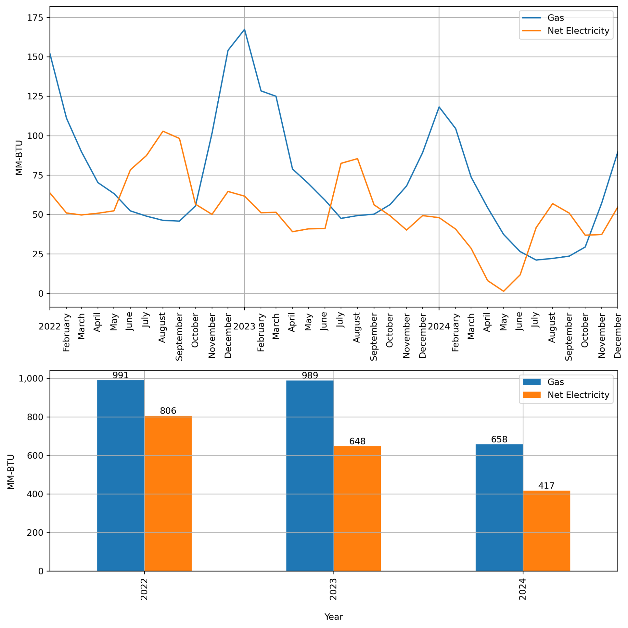
Figure 4. Monthly and annual total gas and net electricity consumption for the entire AH cohort expressed in common energy units (MM-BTU).
Figure 5 provides a more granular view of some of these same temporal trends in energy usage among the AH participant cohort, but instead plots household level consumption time series of both gas and net electricity consumption relative to the timing of the intervention dates for key program measures. The two sub-plots on the bottom of the figure show net electricity and gas consumption trends for each participant household, with the average usage for all participant households plotted as a heavy black line. Likewise, the set of four sub-plots shown at the top of the figure illustrate the timelines of intervention completion dates for each measure type. In these sub-plots the individual dates of completion for each household are shown as gray vertical lines, with the cumulative density of adoptions plotted as a colored shaded area for each. For each of these measure specific sub-plots, the median measure intervention date, e.g. the date by which 50% of program participants had received the measure, is plotted as a thick vertical line. These lines extend down to the corresponding energy usage plots below to give a sense of the rate of progress of implementation for the different types of measures.
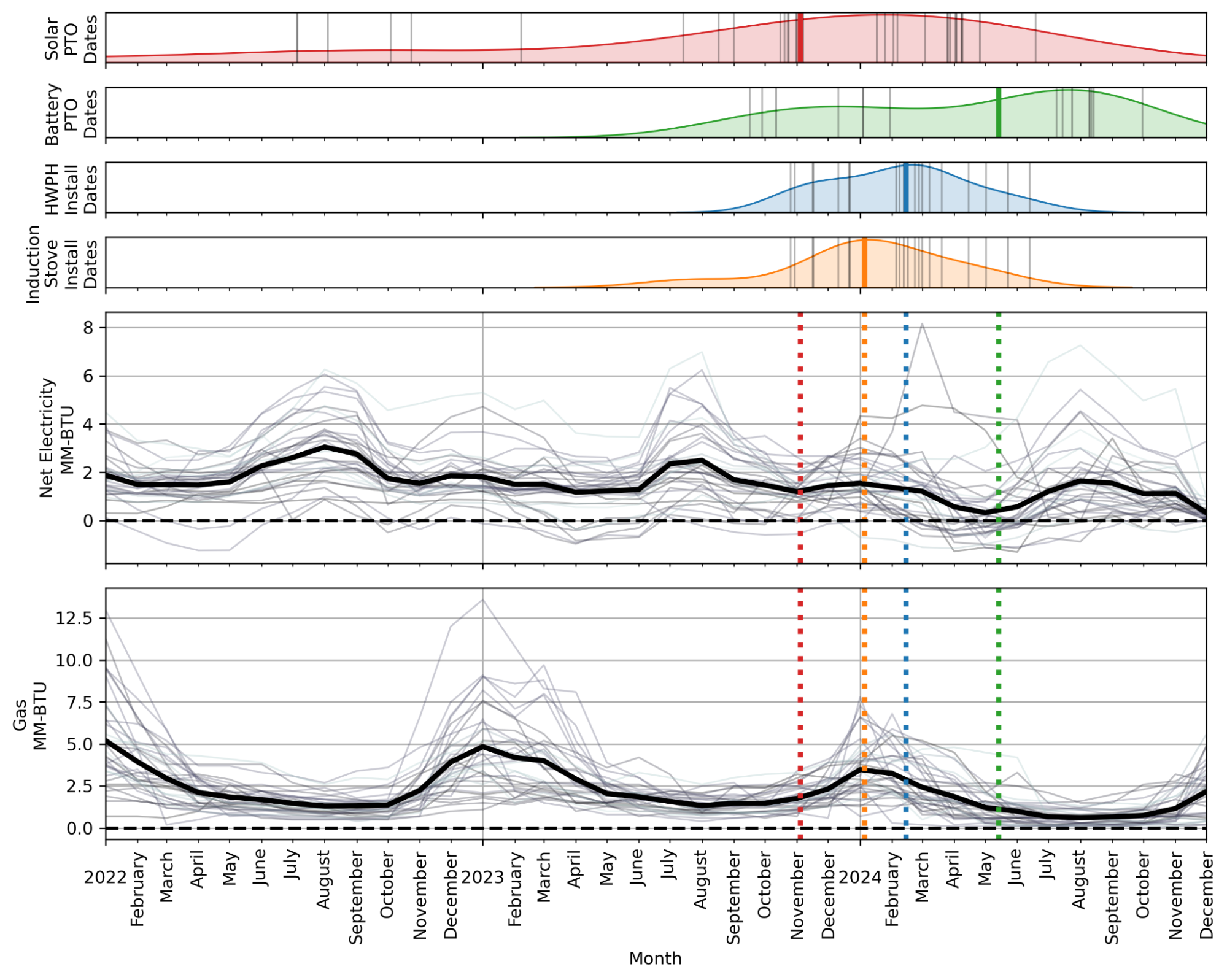
Figure 5. Granular time series plots of individual AH participant household net electricity and gas usage relative to the timing of implementation of different AH program measures. Average household usage rates are plotted as a thick black line relative to each usage time series. Likewise, the median dates of completion for each measure category are plotted as thick colored vertical lines, relative to each measure time series. These median dates are extended as broken lines relative to each usage time series for context. Negative electricity usage values indicate net-exports of power back to the grid.
One feature of note in Figure 5 is the high degree of variability in the monthly gas and electricity consumption levels among AH program cohort households. A portion of this variation can likely be explained by differences in the effective occupancy levels (which were not controlled for) among the homes as well as potential differences in individual preferences/demands for various types of electricity and gas end-use energy services. Another feature of Figure 5 worth noting is that the staggered implementation of different load modifying measures, several of which have strong seasonal effects, need to be taken into account when attempting to evaluate program performance for the full participant cohort. For most of the program participants, the first measure which they received was a rooftop solar PV system, followed later by the potential addition of new electrical loads (HPWHs and/or induction stoves) and ultimately, the installation of a BESS. Variability in the timing and sequencing of these interventions among the participants, which is an unavoidable reality in the implementation of this type of program, makes it challenging to assess the comprehensive effects of the technologies on household energy consumption and expenditures, particularly during the intermediate periods before all of the measures were implemented. We encourage the reader to take note of this feature of the program’s implementation when interpreting these and subsequent findings.
Figure 6, below, seeks to illustrate how different combinations of measures impacted hourly average electricity and gas usage profiles, pre- and post-implementation for the AH program cohort. In the sub-plots on the left-hand column of the Figure, average hourly net-electricity usage profiles for the pre-implementation period are shown as broken orange colored lines. Similarly, average hourly net-electricity usage for the post-implementation period is shown as a solid orange line. Alternatively, in the sub-plots on the righthand column, similar pre- and post-implementation gas usage profiles are shown in blue. Across the rows in the figure, the different sub-plots correspond to collections of program participants who received the same measure package. Finally, within all of the net-electricity usage sub-plots, the timing of the on-peak billing periods associated with SCE various time-of-use rate tariffs are plotted as gray shaded areas.
Relative to changes in electricity usage patterns, there are a number of features worth noting in Figure 6. The first is that for all participants who received battery energy storage systems (sub-plots d, e, f, and g in the figure), net exports of power back to the grid were either significantly reduced or eliminated altogether. Furthermore, in instances where net exports did occur relative to this group, their timing was concentrated around 4-5 PM. This is consistent with a set of battery discharge behaviors that would be expected from an effort to perform arbitrage on time-of-use rate tariffs. The significant reductions in the volume of net exports back to grid indicates that, for a majority of these customers, their solar + battery systems were appropriately sized relative to their loads, such that they could be used to effectively shed on-site demand at peak hours without overproducing. By contrast, for all of the participant homes whose measure packages did not include a battery storage system (sub-plots a, b, and c in the figure), significant net-exports of power were observed over the hours from 7AM - 3PM. This is regardless of whether other measures introducing major new electrical loads were adopted by the home as part of the program. This is problematic as this pattern of loads only contributes to the much maligned “duck curve” - a characteristic pattern of consumption behaviors observable at the system level which demands fast ramping, but typically low capacity factor, generation assets be in place to service the resulting net loads. 6 Relative to changes in gas use, as expected, all of the most significant differences between the pre- and -post implementation periods were associated with participant homes that received some combination of fuel-substitution measures. Here, the most significant reductions in gas use were observed among households who received measure package (c) which consisted of rooftop solar PV, an induction stove, and a HPWH. Here again though, caution should be exercised interpreting some of these pre- and post- intervention changes given the relatively small effective sample sizes involved.

Figure 6. Average hourly electricity (orange, left column) and gas (blue, right column) usage in kBTU for the Pre-Implementation (dotted lines) and Post-Implementation (solid lines) periods aggregated by measure package.
Figure 7 below provides a more granular view of consumption for the AH program participant cohort derived from household level hourly interval meter data. In both sub-plots, the thin stroked lines depicted consumption levels for each individual participant household over each year of the evaluation window (2022-2024). Likewise, the thick shaded lines show the average daily usage levels for all of the participants in the cohort for each year. The sub-plot at the top of the figure shows the full range of variation in these daily average consumption levels across the cohort. In this upper sub-plot, we can see that reported values range from roughly -40 to +45 kBTU per day (with negative values reflecting grid exports). The sub-plot at the bottom of the figure shows a zoomed in view of the same data, but instead focusing on the narrow range of variation in the averages for each year for the entire cohort, -1 to almost 7 kBTU per day.
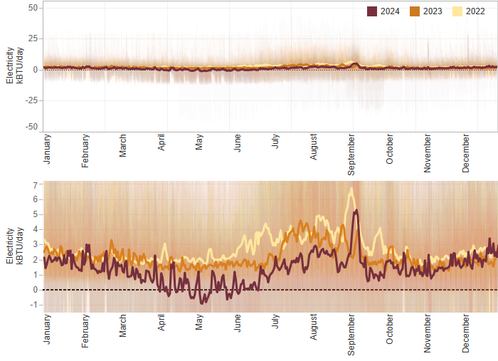
Figure 7. Daily net electricity consumption in kBTU per AH Participant Household colored by year. Average daily net electricity consumption for the entire cohort is plotted in thick solid lines. The top graph features the entire extent of usage while the bottom graph has a truncated y-axis to highlight daily change in the cohort average. Negative usage values indicate net-exports of power back to the grid.
There are several interesting results which can be gleaned from these plots. The first is that even for a small participant cohort such as this (n = 34), the range of variation in individual average daily net-electricity loads can vary 5x more than the average across the entire cohort. This speaks to the level of variability in the energy demands among individual households, even ones which share important structural characteristics, such as those depicted here which all met the eligibility requirements for participation in the AH program. Another important finding visible from these plots is that at the individual household level the largest single day net-exports of power occur in the summer months of August and September. However, across the entire cohort, more power tends to be exported in the spring months of April and May - a trend that is consistent with previously published findings about seasonal variability in the output of residential solar PV systems relative to household electricity demands.7 Here again, the large single day exports for specific customers in those two summer months is due to the work of the battery storage systems discharging for TOU rate arbitrage.
Figure 8, below, plots similar data for the AH program participant cohort’s daily gas consumption. Here again, in the upper sub-plot, we can see that there is an even larger range of variation in household level daily gas usage rates than for electricity. This variation is particularly in winter months with high heating energy demands, suggesting a wide range of variance in the thermal performance of participant homes’ thermal shells as well as in the end-use energy efficiency of their installed gas heating equipment. Looking at the lower sub-plot in this same figure, we can see that the implementation of fuel substitution measures associated with the AH program did not significantly alter the structure of seasonal variation in gas demand between the three years, Rather, these measures appear to have effected uniform demand reductions throughout the entire year (2024). This is consistent with the fact that the program’s two fuel-substitution measures, HPHWs and induction stoves, are not associated with significant seasonal variations in their gas use.

Figure 8. Daily gas consumption in kBTU per AH Participant Household colored by year. Average daily gas consumption for the entire cohort is plotted in thick solid lines. The top graph features the entire extent of usage while the bottom graph has a truncated y-axis to highlight daily change in the cohort average.
Normalized Metered Energy Consumption
Heating and Cooling Degree Hours
To assess the impact of historical variations in weather conditions on energy consumption patterns, historical hourly weather data were obtained from the nearest available official weather station to the project’s eligibility area. These raw temperature data were then converted to heating degree hours (HDH) and cooling degree hours (CDH) using temperature setpoints determined using two-component piecewise linear model fits to actual program participant household electricity and natural gas consumption data (see the discussion related to these fits in the subsequent section as well as detailed fit parameter data provided in Appendices A & B).
For computing HDHs, the temperature threshold derived from pre-intervention AH participant gas consumption data was: 17.72 ℃ / 63.90 ℉. Likewise, for computing CDHs, the temperature threshold derived from pre-intervention AH participant electricity consumption data was: 19.47 ℃ / 67.04 ℉.
The subplot at the top of Figure 9 shows the cumulative number of CDHs (Blue) and HDHs (Red) by month over the project’s time period of evaluation. The subplot at the bottom of the figure shows these same data aggregated on an annual basis. According to these plots 2022 appears to have been an unusually hot year (at least relative to this time period), containing 42% more CDHs than the average number which occurred in 2023 & 2024. This suggests that cooling related energy demands during 2022 should likely have been significantly higher than in the subsequent two years. By comparison, the total number of HDHs across the three years are relatively consistent, only deviating by a maximum of 15% across the three years in the period of evaluation.
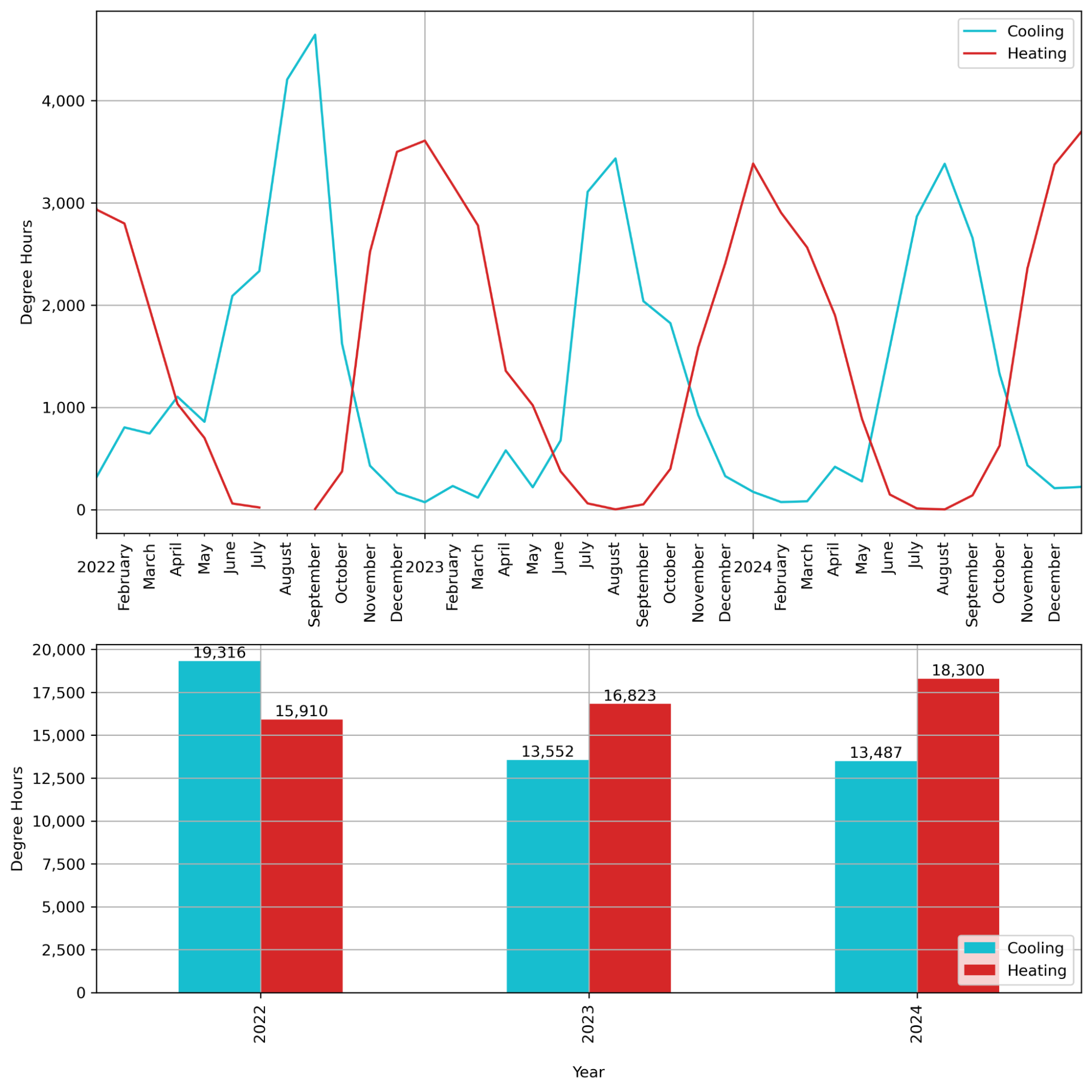
Figure 9. Cumulative total monthly and annual heating degree hours (HDHs) and cooling degree hours (CDHs) for the AH program eligibility area computed using temperature thresholds derived from an analysis of program participant historical energy usage data.
Piecewise Linear Fits of Net Electricity Usage to Temperature
To assess whether the AH program’s measures resulted in normalized metered energy consumption among the participant cohort, a set of two-component piecewise linear models were fitted using electricity usage and historical temperature data for each participant’s pre- and post- periods. The results of these fits are plotted in Figure 10, with pre-intervention period model data and fit shown in Red and post-intervention period model data and fit shown in Blue.
There are several features of note in this plot. Firstly, the pre- period fits exhibit the standard relationship between temperature and energy use, whereby at lower temperature ranges, energy usage is roughly constant (e.g. temperature independent). However, after some threshold temperature breakpoint, incremental demands of energy for cooling creates a positively sloped regression fit component. For the pre- period fit, the identified breakpoint value, after which temperature dependent net-electricity consumption occurs, was found to be 19.47 ℃ / 67.04 ℉. As discussed previously, this was the value used for the computation of CDHs for this analysis.
By contrast, the piecewise fit derived from the post-implementation period data is significantly different. For example, the first component of this fit has a negative slope, indicating increasing net-electricity usage with decreasing temperatures. This is attributable to the significant number of homes which received new HPWHs as substitutes for previously existing gas powered equipment. Additionally, in the post-implementation period fit the breakpoint temperature value identified is significantly higher - at 27.53 ℃ / 81.55 ℉. This is a result of the rooftop solar PV systems’ energy production, with those systems’ outputs being correlated with increased temperatures. Here, the model fit indicates that at temperatures above this breakpoint value, most homes would not be expected to be self-sufficient in terms of power supply and thus would require the net-consumption of additional grid supplied power to supply increasing cooling related energy demands.
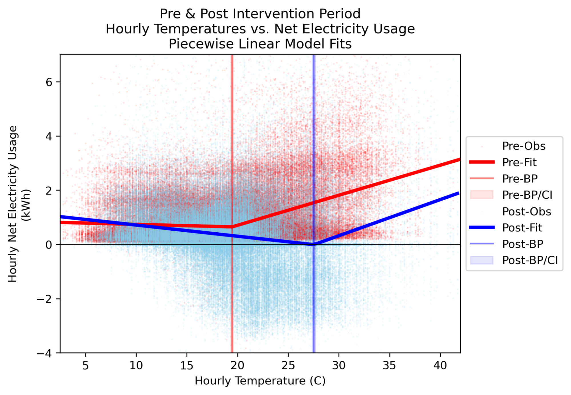
Figure 10. Two-component piecewise linear regression model fit for the relationship between hourly net-electricity consumption and temperature for the AH participant cohort in the pre- (Red) and post- (Blue) program participation periods. The breakpoint temperature threshold for each model is plotted as a solid vertical line with corresponding 95% confidence interval bounds. Negative usage values indicate net-exports of power back to the grid.
Figure 11, below, plots similar results for a set of two-component piecewise linear model fits applied to the relationship between hourly gas consumption and temperatures for the AH participant cohort. Here we can see that the structural characteristics of the relationship between these variables does not appear to have been altered by program participation - which is consistent with expectations based upon the program’s suite of measures. The main effects of program participation on gas consumption are a reduction in the slope of the temperature dependent component occurring at low temperature ranges as well as a reduction in the average magnitude of the non-temperature dependent (e.g. base load) component of participant household gas use in the post-implementation period fit. Both of these can directly be attributed to the two gas fuel substitution measures implemented as part of the program, one of which has a stronger seasonal usage component (the HPWH) and the other of which does not (the induction stove).
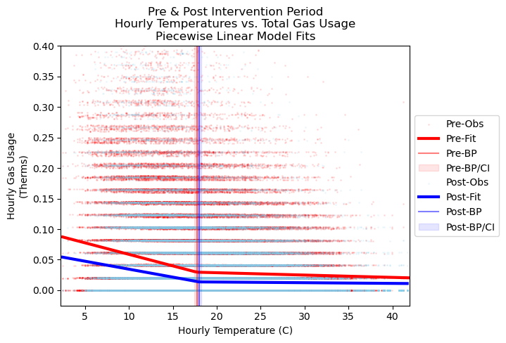
Figure 11. Two-component piecewise linear regression model fit for the relationship between hourly gas consumption and temperature for the AH participant cohort in the pre- (Red) and post- (Blue) program participation periods. The breakpoint temperature threshold for each model is plotted as a solid vertical line with corresponding 95% confidence interval bounds.
Net Greenhouse Gas Emissions Reductions
Interactive Figure 12 describes the absolute changes in daily GHGs associated with both electricity and gas for individual AH participant households as well as the aggregated change for the entire AH program participant cohort. These changes are computed daily to accurately capture values across the variable length pre- and post- implementation periods associated with each individual participant. The sub-plot at the top of Figure 12 illustrates the significant variation in net changes in GHGs that exists at the household level. Despite variation, the data in this plot demonstrates that each participant household experienced net reductions at some point in time during their effective period of performance, with the overwhelming majority of households experiencing total net reductions across the full period-of-performance, and only two households experiencing net emissions increases overall. At the cohort level, greenhouse gas emissions were reduced by a total of 28,184 kg CO2-eq across the cumulative post-implementation periods of performance for all participants. At this cohort level, there were only a small number of individual days in which net GHGs emissions increases were observed. These were generally associated with either extreme high or low temperature periods resulting in high cooling or heating demands - in the case of homes which received new electric water heating equipment. During extreme load conditions, the grid must call into service “peaker” generation assets which can have significantly higher GHG emissions intensities than the average resource mix. These higher marginal emissions intensities can be a more significant contributor to observed GHG emissions increases than changes in the absolute amount of energy consumed over a given period.
While greater reductions for the cohort can be seen in the months of June, July, August, and September, that effect is in part due to a higher number of participant households with available overlapping data between the pre- and post- periods during those particular months. The effects of these limitations in pre- and post- period consumption data availability can be explored in the upper graph by selecting or filtering individual households and examining the timing and duration of their respective periods of performance.
Figure 12. Line graphs of individual and cohort absolute changes in daily total greenhouse gas (GHG) emissions in kg of CO2 equivalent colored from blue (negative changes) to orange (positive changes). The top graph features line graphs of daily absolute change in GHGs for each individual household. Individual participant graphs may be highlighted through selection or filtered using the dropdown menu. The value in the block to the right of the graph displays the total and percent change in GHGs for the selected or filtered participant household for their entire available evaluation period. The bottom graph features the cohort’s total daily absolute change in GHGs with the value block on the right displaying the cohort’s total and percent change for the entire effective evaluation period.
Interactive Figure 13 helps to demonstrate how the variable length of their individual periods of performance contributed to important differences in the calculated net GHG emissions changes across the AH participants. The majority of days available for evaluation are in the months from August to December, followed by summer months. The inconsistency results in an uneven aggregation of GHG changes at the cohort level. This effect is particularly noticeable on certain days in January and February, which show increases in GHGs despite only 6 households with available data.
Figure 13. Plot of the count of AH participants with available days in both the pre and post period (left axis) and the cohort’s absolute change in GHGs for each of those available days (right axis) colored by the cohort’s absolute daily change in GHGs for any particular, available day. Filter the graph based on the measure package using the dropdown menu in the top left or based on the total change in GHGs using the slider in the top right.
The histograms provided in interactive Figure 14 illustrate the distributions of the relative and absolute changes in daily GHGs with an emphasis on the different measure packages adopted. Both plots feature fairly normal distributions whose centers reflect overall net reductions in GHGs. This feature is consistent at both the full cohort level as well as among the individual measure packages. The centers of these component distributions generally reflect the distribution of the measure packages across the cohort (a greater number of GHG reduction days for measure packages in which more households partook).
Figure 14. Histograms of relative (left) and absolute (right) change in daily total GHG emissions by AH participant household and colored by measure package. Selecting a block in the histogram will highlight all relevant measure packages. Hovering over blocks in the histogram will reveal their exact change values. Use the dropdown menu in the top left to filter to specific measure packages and use the dropdown in the upper right to view all measure packages in one histogram or to view each measure package separately.
Figure 15 below plots daily greenhouse gas emissions from net-electricity usage (left), gas (center), and net-electricity + gas usage (right) for the entire AH participant cohort. These heatmaps illustrate changes in GHG emissions at different times throughout the year. At the cohort level, we can see significant GHG reductions occurred between 2022/2023 and 2024, the year which most closely coincides with full implementation of all AH program measures. Relative to the gas combustion related GHG emissions depicted, it is worth noting here the daily variations shown essentially reflect daily changes in gas demand. This is because a constant GHG emissions factor was used in this case. By contrast, the daily variations in GHG emissions from electricity reflect temporal changes in both the net consumption and emissions intensity of grid electricity.
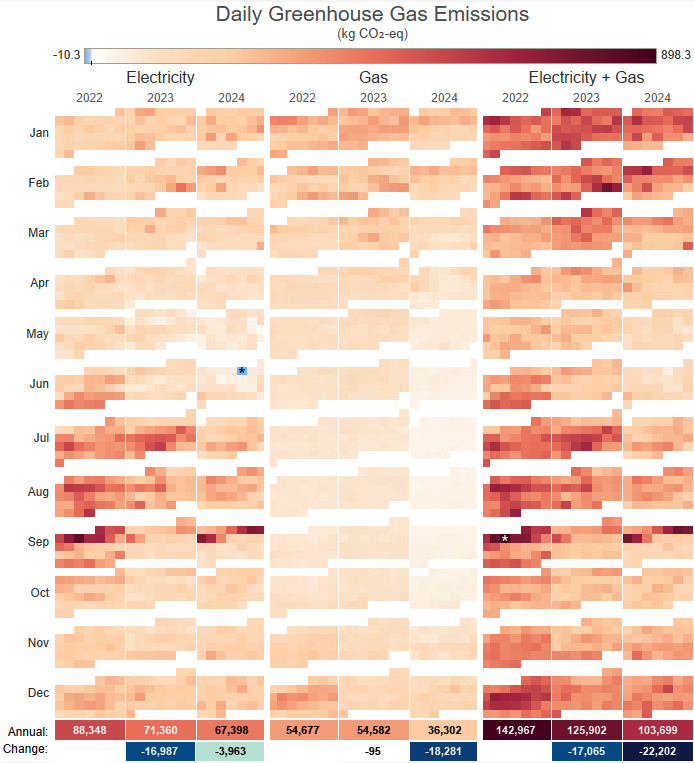
Figure 15. Heatmaps of daily Greenhouse Gas (GHG) emissions in kg of CO2 equivalents for the AH program participant household cohort. Negative GHG values (in blue) indicate net reductions in GHGs due to exports of electricity back to the grid. Positive GHG values are colored by an orange-red gradient. The minimum cohort daily GHG value is indicated with a black asterisk (June of 2024, Electricity) and the maximum value is indicated with a white asterisk (September of 2022, Electricity + Gas). The bottom two rows of values represent the annual GHG totals (top) and the change in annual GHG totals from the previous year (bottom).
Interactive Figure 16 provides a similar view of household level daily GHG emissions except for each individual AH participant. These plots illustrate key measure implementation dates and can be filtered according to distinct measure packages. They also provide estimates of individual household level annual GHG emissions reductions.
Figure 16. Heatmaps of daily Greenhouse Gas (GHG) emissions in kg of CO2 equivalents for individual AH program participant households. Negative GHG values (in blue) indicate net reductions in GHGs due to exports of electricity back to the grid. Positive GHG values are colored by an orange-red gradient. The bottom two rows of values represent the annual GHG totals (top) and the change in annual GHG totals from the previous year (bottom). Intervention labels indicate the PTO or install date for each of the participant’s measures (S-Solar, B-Battery, H-HPWH, I-Induction Stove). Selections in the top two dropdown menus will filter and update the heatmaps. Hovering over a particular day in the heatmap will reveal the date and the total GHG value for that day.
Energy Bill Savings
Among the key-performance indicators being evaluated for the AH program was the extent to which total energy bill savings would be realized for the participant households. The types of bill savings are challenging for program implementers to accurate forecast for individual households prior to program participation, due to the unpredictable nature of the occupants interactions with fundamentally new technologies with different performance characteristics from the incumbent systems which they replaced, and in some cases, which offer fundamentally new types of energy services that may not have been previously accessible.
The subplot at the top of Figure 17 shows the distribution of total monthly net-electricity and gas bill expenditures for the full AH participant cohort over the project’s evaluation period. The subplot at the bottom of the figure shows these same data aggregated on an annual basis. There are a number of features on note within this plot, particularly when compared to the information for total energy usage depicted in Figure 4, previously. Firstly, across the entire evaluation period AH program participants spent significantly more on electricity than on gas. This is despite using significantly more gas, in absolute energetic terms. This is a consequence of the significant price premium which must be paid per unit of energy in the form of electricity, as compared to gas - as well as factoring in electricity’s dynamic time-of-use rate structures.
In the two years which roughly correspond to the pre-implementation period for most participant households - 2022 & 2023 - the AH program cohort’s electricity expenditures were 65% and 52% greater than their corresponding annual gas expenditures, respectively. Here we must keep in mind previous observations from the analyses of historical weather data, which revealed 2022 to be a particularly warm year, likely resulting in larger than normal cooling energy demands. However, as we shall subsequently detail, a counterbalancing factor in this calculation was an anomalous gas commodity price spike in January of 2023 which significantly inflated overall gas expenditure levels for that year.
In the final year of the project evaluation period - 2024 - which roughly corresponds to the post-implementation period of performance for most participant households - electricity represents a 68% share of total energy expenditures, the largest ratio of any of the three years. Overall, when factoring changes in expenditures across both fuels, at the cohort level, there was a 43% reduction in total combined energy bill expenditures in 2024 relative to the average of similar totals computed for 2022 and 2023.
When taken together, these findings indicate that the AH program’s measure packages were effective at significantly reducing total combined energy expenditures at the cohort level. And though the proportional share of remaining expenditures shifted somewhat from gas to electricity, the significant increases in the efficiency of the new substitute electrical technologies was more than sufficient to offset the significant price differences between gas and electricity per unit of energy consumed.

Figure 17. Monthly and annual total gas and net electricity expenditures for the entire AH cohort expressed in dollars-$.
An important feature of note in Figure 17 that warrants further discussion has to do with the appearance of negative expenditures for gas in the month of April for both the 2022 and 2024 data years. These negative expenditures occur due to the gas utility’s disbursement of California Climate Credit funds, which are the result of net-proceeds of the state’s GHG emissions cap and trade program. These funds appear as an on-bill credit for qualifying customers each year at this time. For these two years, the size of these credits were more than sufficient to offset the cohort’s total gas bills, resulting in net payments. 2023 is somewhat anomalous in this regard as this characteristic dip in April is not present. We believe that this is due to a significant spike in the commodity price for gas which occurred in January 2023. This price increase is well illustrated by the plot in Figure 18, below, which shows the SoCal Gas resource procurement rate over the project’s period of evaluation. In January of 2023, due to commodity market conditions, this procurement rate increased to ~5x from previous historical levels. These resource procurement rates have since stabilized to levels that are even somewhat lower than those observable prior to January of 2023.
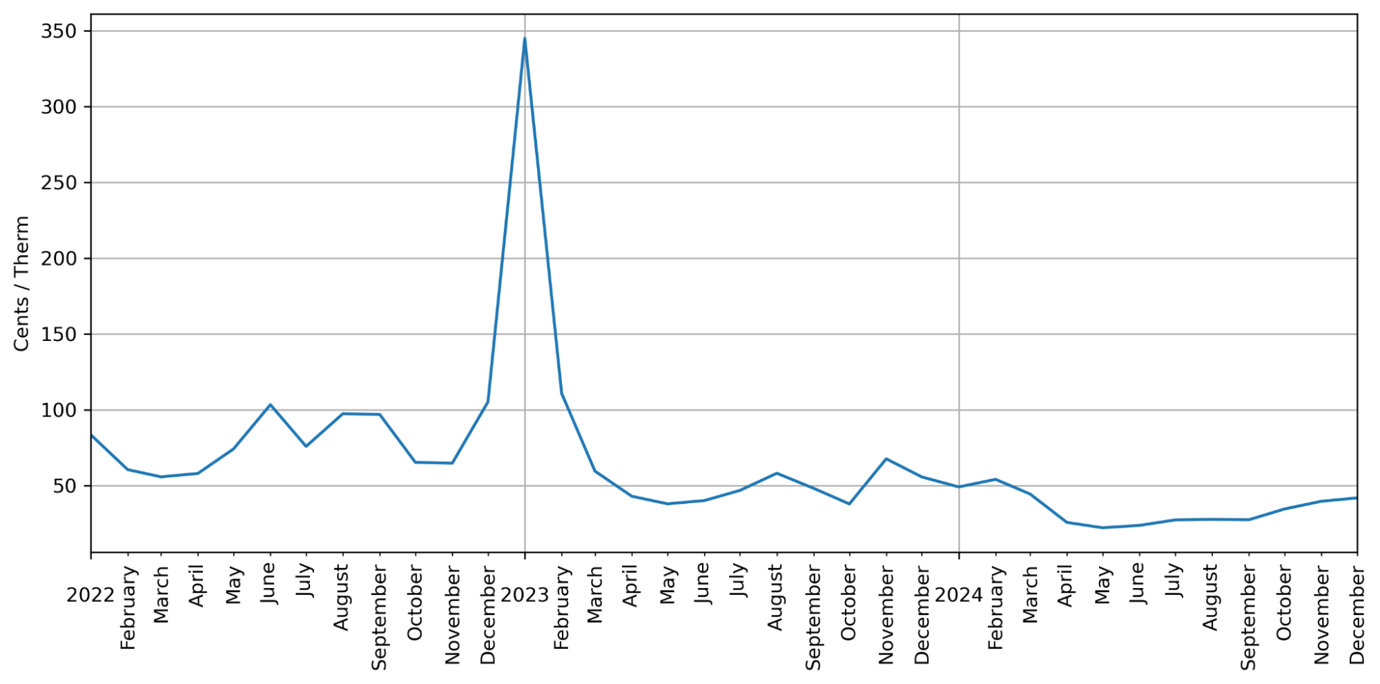
Figure 18. SoCal Gas resource procurement rate (cents per therm) over the BAAEC AH program implementation period.
Figure 19 below provides a more granular household level view of AH program participant electricity and gas bill expenditures, presented in a similar format to that previously provided in Figure 5 for household energy use. Here again, the timing of different program interventions is plotted for context. It is perhaps worth noting that the variability in bill expenditures between participant households is much greater for net-electricity usage than it is for gas. As household size (e.g. number of occupants) is not implicitly controlled for in this comparison, it is likely that these differences are, at least in part, attributable to the role of dynamic pricing for electricity and the effect which that has upon different individual households’ bills due to their characteristic temporal patterns of consumption.
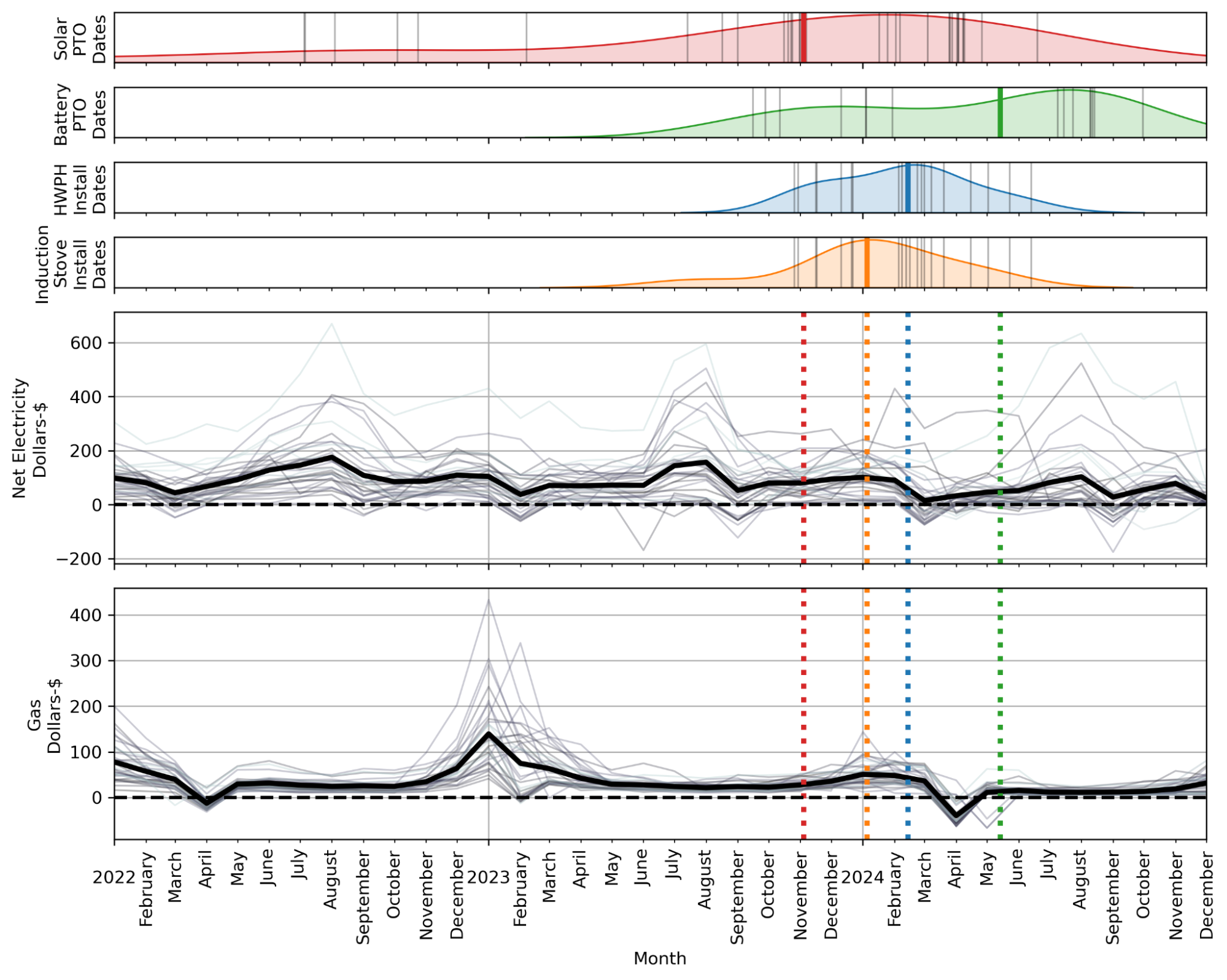
Figure 19. Granular time series plots of individual AH participant household net electricity and gas expenditures relative to the timing of implementation of different AH program measures. Average expenditures, across all households, are plotted as a thick black line relative to each usage time series. Likewise, the median dates of completion for each measure category are plotted as thick colored vertical lines, relative to each measure time series. These median dates are extended as broken lines relative to each usage time series for context.
The series of sub-plots in Figure 20, below, attempts to tell the complete story of gas and electricity bill savings resulting from households’ participation in the AH program. The three sub-plots in the upper portion of the figure depict a series of box-plots which capture the electricity, gas, and total combined bill savings calculated between the pre-and-post intervention periods for each household for each month. The sub-plot at the bottom of the figure provides a bar chart which depicts the percentage of program participant households for whom their specific pre-and-post period dates permitted the making of such comparisons for each month. In other words, this sub-plot shows how the effective sample size associated with the corresponding box-plots is not uniform across the months - with fewer savings comparisons being able to be made in the earlier portion of the year. The inset text boxes positioned to the right-hand side of the three upper subplots provide important summary statistics about the average savings for each associated category of energy expenditures.
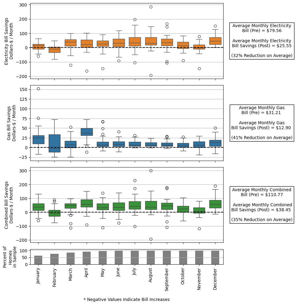
Figure 20. Distributions of calculated net-electricity, gas, and total combined bill savings by month for each participant household (for which data were available) for each month of the post-implementation period. Negative dollar values indicate instances of assessed bill increases from the pre-implementation period.
Overall, as shown in Figure 20, the typical household experienced a $25.55 reduction in average monthly electricity bills (-32%) and a $12.90 reduction in average monthly gas bills (-41%) as a result of their participation in the AH program. When combined, this equates to an overall savings of $38.45, on average, in total monthly energy expenditures (-35%). Here again, we would expect these numbers to be slightly different if a full year of post-implementation period expenditure data were available for each household for purposes of evaluation. However, it is unlikely that the availability of such data would so significantly alter the results that the main conclusions, that the program having resulted in significant net bill savings for the average participant, would have to be altered.
There are a couple of additional issues worth noting relative to the interpretation of these calculated bill savings amounts. The first is that prior to their enrollment in the AH program, only 17 of the 34 participant households (50%) were already enrolled in dynamic, Time-of-Use (TOU), electricity rate tariffs. All AH participants who received solar PV systems were necessarily transitioned to new TOU rates as part of the interconnection process. This means that, depending upon each individual household’s load shape, the switch to TOU rates could have independently impacted their bill amounts, without any changes in their energy consumption patterns what-so-ever.
Additionally, through the course of the program’s implementation period the CPUC transitioned from a Net-Energy-Metering (NEM-2.0) to a Net-Billing (NEM-3.0) tariff. This change significantly altered the levels of financial compensation for power being exported back to the grid by small scale, distributed PV systems. Which of these two tariffs AH participants were allowed to access depended upon the timing of their specific interconnection applications. As a result, 10 of the 34 AH participant households (29%) were able to be enrolled under the more favorable, NEM-2.0 tariff. The remainder were enrolled under the NEM-3.0 Net-Billing Tariff, whose structure significantly favored the installation of BESS in conjunction with solar PV.
Net-Zero Electricity Status
Figure 21, below, plots the ratio of grid electricity deliveries to exports for each AH participant household (light shaded lines) as well as the average for the entire participant cohort (dark shaded line) over the project’s evaluation period. Here, it is worth noting that the different household level data series begin at different points in time. This is due to the fact that type of net calculation can only be performed once their solar PV system had been installed and thus net-exports were possible. The broken horizontal line plotted at 100% depicts the threshold cutoff associated with the achievement of net-zero electricity status. Here we can see that while many individual households were able to achieve this status at some stage, none of them were able to sustain it continuously through the end of the evaluation period. At the cohort level, there were similarly some individual months over which net-zero electricity status was achieved, on average, across all participants. However, this was similarly not able to be sustained for more than months in succession.
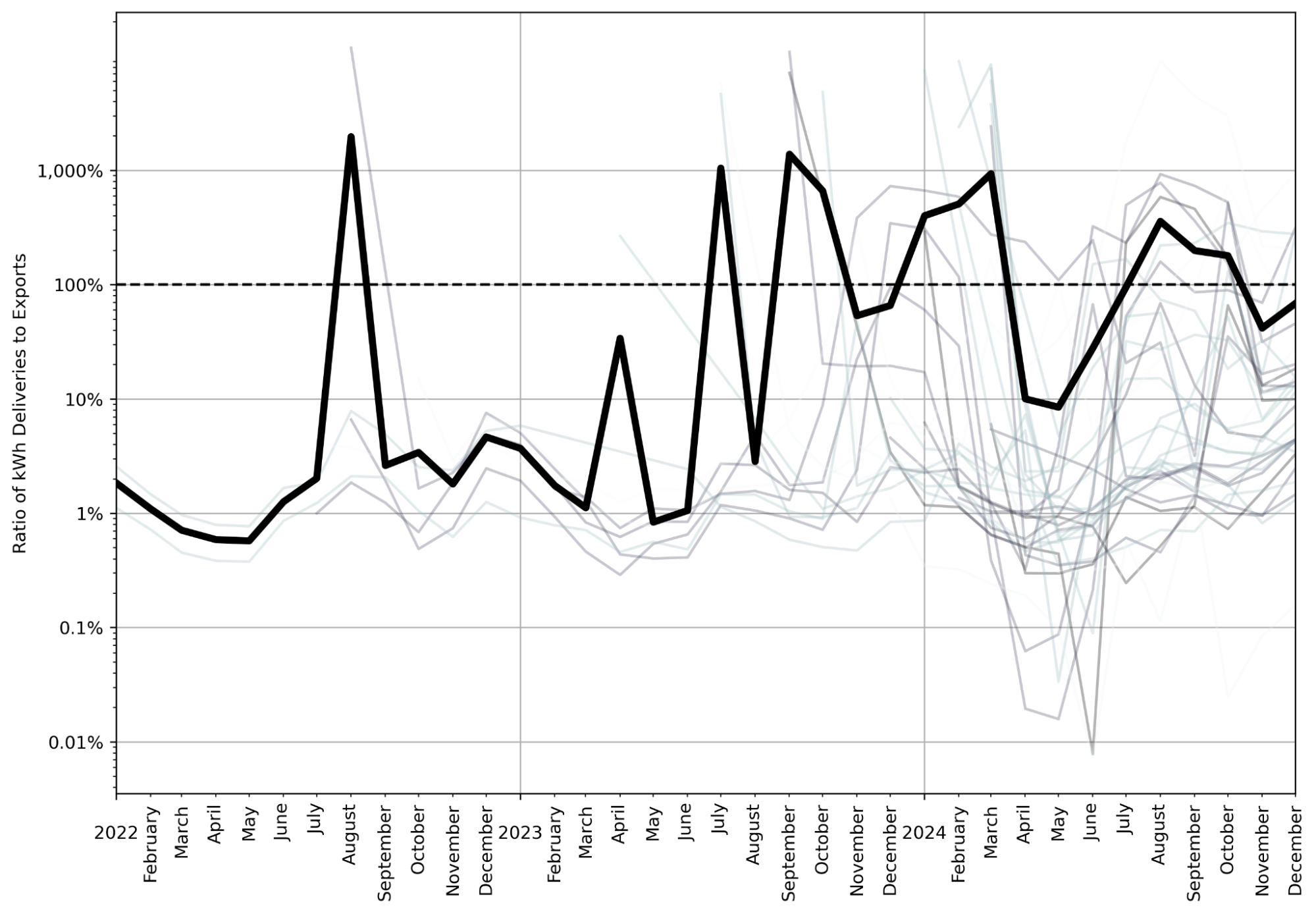
Figure 21. Ratio of grid electric power deliveries to exports for each month in the project evaluation period. The light shaded lines reflect individual households, while the thick black line reflects the average for the cohort as a whole. The staggered appearance of individual household data reflects the variable timelines of solar PV system installs across the cohort. The broken horizontal line corresponds to the threshold ratio corresponding to net-zero electricity status.
Interactive Figure 22, below, plots similar data for the number of AH program participant homes that achieved net-zero electricity status over the course of the project’s evaluation period, only instead at a daily time interval. Here we can see the highest concentration of participants were able to successfully net-out the daily grid electricity consumption in the months of April, May, and June. For a subset of the days within these months as many as 18 of the 34 homes achieved net-zero electricity status.
Figure 22. Heatmap depicting the daily count of AH participant households that reached net-zero electricity status within each of their respective post-intervention periods. The lightest green color represents a single AH participant household reaching net-zero electricity status in a day while the darkest green represents a maximum of 18 AH participant households reaching net-zero electricity status in a single day (indicated with white asterisks). Hover over a date to view the exact count of AH participants that reached net zero on that day.
Figures 23 and 24, below, provide a different perspective on these same daily net-zero electricity attainment count statistics, depicting the total number of days achieved according to the different combinations of measures received by the participant households and the percentage of post-implementation period days over which net-zero status was attained, respectively. Interestingly, the individual households which achieved the largest number of net-zero electricity days over the project’s evaluation period were those which only opted to receive solar PV systems through the program. There are a number of potential explanations for this fact, however the effective sample size of this sub-group is so small that it cannot be considered a statistically significant finding.
Another interesting feature of this plot is the fact that the homes with the smallest number of days over which net-zero electricity status was attained were all those which opted for fuel-substitution measures as part of their participation in the program. This can perhaps be explained by the fact that solar PV system sizing guidelines are based upon meeting, but not exceeding, 150% of each customer’s historical energy loads.
Rooftop PV system sizing is a process that must respect various site-specific constraints - from roof size and orientation, to sources of shading and other obstructions. Based upon internal data collected by Grid Alternatives, we can report that the average AH program participant’s PV system was able to be sized to meet 91% of their historical on-site loads. These systems represented 3.96 kW-AC of nameplate capacity, on average. If significant new loads were introduced after a participant’s system had been installed, they may be insufficiently sized to reliably net-out the future demand for grid electricity. Of course, with this, as with all of the analysis discussed in this report, it is important to keep in mind the potentially confounding effects of variations in the periods of performance for each household, as previously discussed.
Figure 23. Count of days of net zero electricity status per AH participant household, colored by intervention and bins of 30 days. Hover over an element to view its summary.
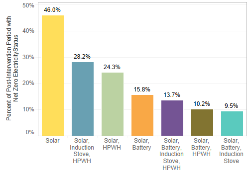
Figure 24. Bar chart comparing the percent of post-intervention days in which households across intervention configurations achieved net zero electricity status.
Conclusions
Key Findings
Acknowledging the significant limitations to this EM&V analysis discussed throughout the report stemming from the small program participant cohort size, heterogeneous measure packages, variable implementation timelines, and limited temporal scope of available consumption data from the IOUs - there are still several important findings which can be taken away from the evaluation of the AH program relative to the high-level objectives of the Advanced Energy Communities grant funding opportunity’s research objectives. These include the following.
-
Fuel-substitution measures such as HWPHs and induction stoves can confidently deliver significant reductions in overall customer energy expenditures and net-GHG emissions when implemented in conjunction with distributed energy resources (e.g. solar PV + battery energy storage systems). Overall, the AH program’s participants, on average, experienced a 35% reduction in combined annual electricity and gas bills and a 923 kg reduction in combined GHG emissions as a result of their participation.
-
A majority of the program’s participant homes were able to achieve net-zero status, but only for a minority of the months in their respective post-implementation periods. For many of these households, the addition of new electrical loads associated with included fuel-substitution measures likely played a role in this fact. Current PV system sizing guidelines are oriented towards netting-out historical energy demands.
-
Net-zero electricity status is possible to achieve with the combination of measures involved with the AH program. However, this may not be the most useful metric of performance relative to both the priorities of the grid and those of individual customers. Evidence suggests that most AH program participants were principally motivated by the possibility of energy bill savings. Likewise, from the power system’s perspective, program participant measures which delivered net-electricity reductions during peak period hours, or otherwise maximized net-GHG emissions reductions, may be considered more meaningful than the achievement of net-zero electricity status by other means.
-
By default, most BESS controls do not pursue the objective of achieving net-zero electricity status. They are instead trying to maximize energy bill savings from their operations to accelerate the production of benefits for the program’s participants in terms of electricity bill reductions. These equipment would likely require different modes of operation, and potentially, access to new sources of market or infrastructure information, in order to maximize GHG emissions reductions or grid electric energy usage reductions, for example. These different control strategies have important implications for the alignment of dynamic electricity prices, and other market signals, with state energy policy objectives.
-
**There are important tradeoffs in terms of a BESS’ ability to provide different classes of benefits and their ability to provide a reservoir of available back-up power, on-site, in the case of an outage. This hints at broader questions about whether and how distributed energy resources should be operated to maximize benefits delivered to the customers and local communities which host them (e.g. bill reductions & back up power capacity) versus the collective benefits of the system which they are a part of (e.g. provisioning of grid services & facilitating GHG emissions reductions). **
Discussion
Program Implementation Challenges
One of the main themes of the BAAEC project’s implementation phase has been the compounding challenges associated with the attempting to implement a set of advanced fuel-substitution and distributed energy resource measure packages within low-income, disadvantaged community households. This is in part because these households face a myriad of structural challenges to not only their participation in complex programs but also to their physical capacity to receive these types of technologically advanced systems. Generally, households like those which were targeted for participation in the AH program have a low tolerance for:
- Bearing any additional costs associated with required site remediation work
- Taking time to host multiple in-person site visits for property inspections for system design work and program eligibility verification
- Accommodating uncertainties in the long term bill impacts (e.g. risking cost increases) from installed measures
Added to these challenges facing the program’s eligible participants were other challenges facing program implementation partners seeking to deploy new technologies or implement fundamentally new business models. A detailed narrative discussion around the interplay of these forces over the course of the AH program’s implementation period is provided in the project’s Case Study report. However, it is perhaps sufficient to say here that the net effects were significant delays in the implementation of certain program measures - most specifically for the BESS - as well as reductions in the number of homes who were able to be enrolled in the program relative to levels that had initially been targeted in its conception. Both of these outcomes played important roles in our ability to derive concrete, statistically significant, findings within the scope of this EM&V analysis.
Finally, in order to better accommodate the specific needs, as well as structural barriers, facing eligible AH program participant households, the decision was taken to design the program as a suite of optional measures. While this decision was useful in accommodating potential participant households, it created fundamental comparability challenges for this type of EM&V analysis - as an already small cohort of participant households (34 total) would need to be further subdivided according to seven distinct measures packages in order to make direct, apples to apples, comparisons.
Data Accessibility Challenges
A significant barrier to the EM&V analysis developed in this report was the availability of historical consumption data from SCE and SCG over a long enough time period to span the full implementation of all of the program’s included measures. Specifically, both SCE and SCG referenced specific challenges associated with pulling customer interval data for more than three years prior to the date at which data requests are submitted. These challenges stem from data archival practices that are implemented to comply with corporate data retention policies. We recommend that CPUC provide guidance to the state’s IOUs about what the appropriate retention periods should be for customer usage data. The goal here should be to provide clarity to parties submitting data requests through the EDRP as to which requests should and should not be easily fulfilled such that they are not surprised by delays associated with accessing data that has been moved to archival formats or may even have been permanently deleted.
Another significant barrier for this type of analysis has to do with uniquely identifying customer premises across separate, single-fuel utilities, such as SCG and SCE. Each utility’s backend data systems have their own customer account information and premise identification codes. These must be reconciled to reliably request gas and electricity consumption data for the same cohort of customers. The state would be well advised to pursue the development of a unified customer premise identification code that could be used as a shared key, amongst these single-fuel utilities, to better link siloed customer datasets and improve the experience of conducting this type of fuel-substitution program analysis going forwards.
Community Solar (CS) Program
Background
The BAAEC project’s Community Solar (CS) program involved the construction of two medium sized (400 kW-AC & 270 kW-AC) solar PV systems on the rooftops of a set of adjacent self-storage facilities in the city of Pico Rivera. These sites were selected because they were within 5 miles of the original set of four disadvantaged community census tracts that constituted the BAAEC project’s initial focus area. The project developer was Pivot Energy (Pivot). Pivot and TEC worked closely on submitting an application to the local Community Choice Aggregator, the Clean Power Alliance (CPA), as an eligible generation site under its pilot Community Solar Green Tariff (CSGT) program. This is a program, initiated by the CPUC, using ratepayer funding, that is intended to benefit residential customers (with at least 50% of project’s output subscribed by customers eligible for CARE or FERA utility discounts), including renter households and those living in multi-family properties within Disadvantaged Communities. These types of customers have been identified as a priority for these types of community solar programs as they would otherwise have a very difficult time accessing the benefits of solar net-billing tariffs.
Program Design
Enrollment
The CPA, as the implementor of this new CSGT, initially specified a set of customer eligibility criteria that involved a voluntary enrollment process. This placed the burden of proof for demonstrating program eligibility on interested customers. Throughout the evolution of the project however, and after many BAAEC community solar subscribers were recruited, CPA changed this process to allow for auto-enrollment of customers based upon a set of revised eligibility screens that could independently be applied by the CPA itself.8 These included known customer attributes such as location, historical electricity usage levels, and billing arrears amounts. For future programs, this new auto-enrollment procedure will dramatically reduce the transaction costs associated with outreaching to potentially eligible customers, educating them of the merits of the program, and convincing them that it was worth their time to go through the process of submitting an enrollment application. Table 3 summarizes the key characteristics of CPA’s CSGT program.
Table 3: Key characteristics of the CPA’s CSGT Program
| Customer Eligibility Requirements | Residential customers in DACs & 50% of a project’s output subscribed by customers eligible for CARE or FERA |
|---|---|
| Participating Customer Benefits | 100% renewable energy & 20% off their otherwise applicable electric rate |
| Project Location Requirements | In DACs within 5 miles of DAC(s) where subscribing customers reside |
Figure 25, below, shows the location of the two adjacent BAAEC CS sites located within the city of Pico Rivera. A five mile buffer (red) has been plotted around the two sites. The intersection of this buffer and the CPA service territory (purple) can generally be regarded as the geography which contains the set of CPA customers that would be considered eligible for enrollment in the CSGT as part of the project - though obviously, in addition to this, other individualized screens would apply. As the figure shows, this buffer area intersects with the four census tracts that were originally designated as the BAAEC project’s eligibility area (though this was later significantly expanded). While representatives of the CPA indicated that they do specifically associate individual CSGT participant customers with specific generation projects, we do not know who these customers are and how many of them may specifically be located within the BAAEC tracts. This is a fundamental limitation of the data available for this analysis and a consequence of the CPA’s customer privacy protection.
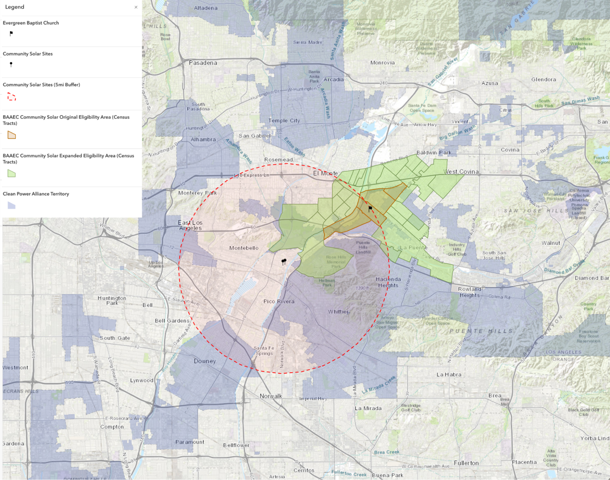
Figure 25. Map illustrating the location of the two BAAEC Community Solar generation sites relative to the location of the project’s original and subsequently expanded focus areas, as well as the boundaries of Clean Power Alliance’s service territory.
Measures
Enrollment in the CPA’s CSGT program requires no physical alterations to a participant’s property or the installation of any on-site equipment. All physical interventions were localized to the community scale generation facilities enrolled as part of the project. The output of these community solar assets are virtually allocated to CSGT participant customers by reducing their bills by a fixed percentage amount (-20%). In this way, the CS system’s outputs are allocated to customers participating in the program in a manner that is proportional to the volume of their consumption.
Terms
Beyond initial enrollment, the only customer obligation for participation in CPA’s CSGT program involves the continued verification of income eligibility for CARE/FERA assistance programs. If customer incomes increase above this eligibility threshold or they fail to verify this eligibility on a regular basis, it is possible that they may be dropped from the program. CPA staff make efforts to notify customers who may be at risk of this type of disenrollment so that they can obtain the required income verification. Customers are only disenrolled and stop receiving VNEM benefits under the program if they fail to obtain this verification after a period of several months.
Methods
Data Sources
Southern California Edison (SCE)
The same sample of customer interval usage data which was obtained for use in the EM&V analysis for the AH program scope was also used here to evaluate the performance of the BAAEC CS system. We encourage the reader to reference the documentation for the stratified random sampling procedure that was used to construct this customer sample that is documented in that earlier portion of this same report.
Control Group Customer Sampling
In an effort to minimize the amount of sensitive utility customer data requested for this control group, a stratified sample of 8,000 SCE customers was developed. This sample was constructed by filtering on a key set of attributes that related to CS program eligibility. These sampled customers were selected from a group of 37 zip codes located in proximity to both the CS program’s eligibility/recruitment territory. This control sample of customers were partitioned according to the following criteria:
- CARE/FERA Assistance Program (50% Enrollees / 50% Non-enrollees)
- Single-Family & Multi-Family Premises (50% SF / 50% MF)
- Clean Power Alliance (CPA) (50% Enrollees / 50% Non-enrollees)
- CalEnviroScreen Disadvantaged Community (50% Members / 50% Non-Members)
This stratified random sample was designed such that there would be 500 distinct control group customers within each strata. These strata are defined as all of the unique pairwise combinations of the binary attributes listed above. Based upon the number of strata involved, this yielded a full control group sample of 8,000 customers. Ultimately however, this report’s analysis principally made use of sampled historical meter data for the subset of customers who were: CPA members, CARE/FERA enrollees, and located within DAC census tracts. All of the subsequent analysis shown is based on this group of potentially eligible participants, partitioned only by their SF versus MF status.
Pivot Energy
The project manager at Pivot Energy responsible for developing the BAAEC CS sites provided the UCLA research team with relevant details about the design characteristics of the project site that were necessary for conducting this EM&V analysis. These details included the BAAEC project sites nameplate capacities (kW-DC) and inverter output ratings (kW-AC) as well as hourly interval production data for several other sites that could be used as a point of reference for the analysis.
Clean Power Alliance
The program manager at the Clean Power Alliance responsible for administering the CSGT provided the UCLA research team with relevant details about the anticipated monthly energy energy consumption of potential program enrollees. This number was used internally by the CPA to determine the number of enrollees that would be specifically tied to the output from the BAAEC CS generation sites. Specifically, it was communicated to us that the average monthly energy consumption assumed for eligible customers was estimated to be 408 kWh / month. This resulted in a BAAEC CS program cohort cap of 360 total customers.
Modeling PV System Outputs
Due to delays associated with the construction and grid interconnection of the actual BAAEC CS generation sites, they were not able to receive permission to operate until after the window of IOU customer data availability used for this EM&V analysis closed. Consequently, the decision was taken to use another Pivot Energy developed site - of similar size, located within close proximity to the BAAEC CS generation sites, which was operational over the desired period of performance - as a proxy reference for determining what the BAAEC sites output would most likely have been were they operational. Hourly interval production data for several candidate proxy sites were provided by Pivot Energy, of which, one was selected for use in this analysis.
The proxy site which was selected has a nameplate rating capacity of 106.08 kW-DC under standard test conditions. This DC nameplate capacity is derated to 74.88 kW-AC based upon the system’s installed inverters capacities and configuration. This latter value was used to establish a normalized hourly output factor (kWh / kW-AC * hour) for the proxy site. This value was then multiplied by the combined BAAEC CS systems’ nameplate rating (670 kW-AC) to derive a modeled BAAEC CS generation output time series dataset (kWh / hour). Subsequent reported results are based upon a detailed analysis of this modeled output.
Results
Modeled System Outputs
Figure 26, below, plots the modeled output of the BAAEC system over the project’s full period of evaluation aggregated at hourly (top) and monthly (bottom) intervals. Note that the specific period of performance that will be used for subsequent EM&V analyses is the 2024 calendar year. As Figure 26 illustrates, based upon the hourly output of the proxy system, we anticipate that the BAAEC CS sites would have output between 47 and 138 MWh per month in 2024. Annually, this expected system output would total to 1,163 MWh for 2024. This value is thus the basis of comparison for the evaluation of the system’s capability to effectively net-out the electricity consumption of CSGT program enrollees.
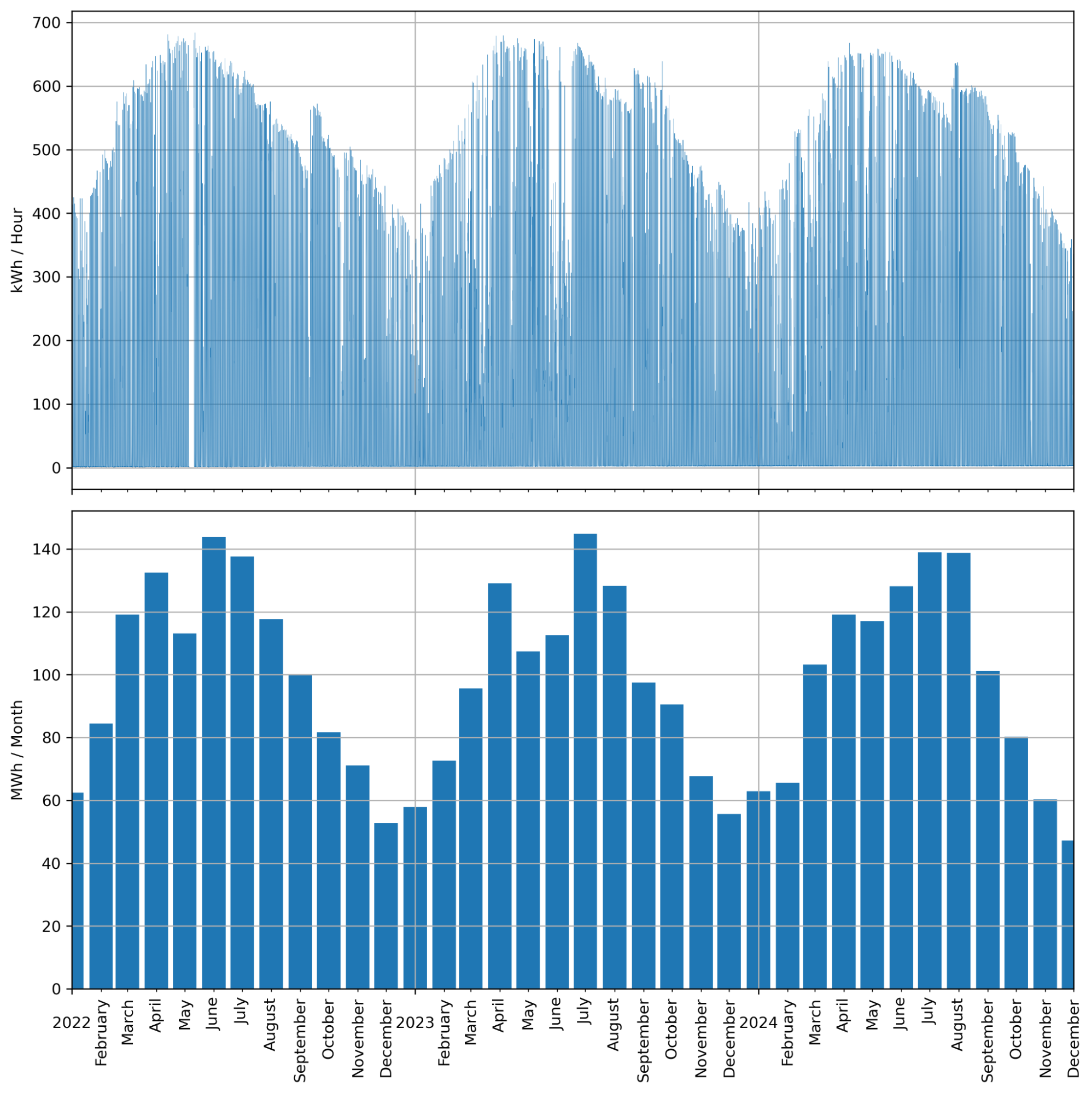
Figure 26. Modeled BAAEC CS system output based upon scaled output data from another Pivot Energy proxy system collected over the project’s full evaluation period.
Net Zero Electricity Status
Because we do not know which specific CPA customers enrolled in the CSGT program were associated with the BAAEC CS systems, we need to rely on statistical approaches to evaluate the loads that would likely be associated with a cohort of customers of the size prescribed by the CPA (n = 360). To do this, we developed a Monte Carlo Sampling procedure using the sample of customer level electricity usage data that was obtained from SCE through our EDRP request.
Figure 27, below, provides a set of fan plots that illustrate the distribution (shown at 5 percentile increments) of monthly electricity usage among CSGT eligible single-family (red) and multi-family customers in our sample data. In both sub-plots the cohort median (across all months) is plotted as a black broken line, while the fixed monthly usage value used by CPA in the program’s design (408 kWh / month) is plotted as a black solid line.
There are a number of notable features in these plots. Perhaps most significant of which are the significant differences in the range of monthly usage values between single-family and multi-family customers. Multi-family customers, on average, use only about half of the electricity each month as their single-family counterparts. In addition to this, we can also see that the CPA’s estimated average monthly usage value is just a bit lower than (-11.88%) the observed median (~463 kWh/month) for eligible single-family households in our data sample. Looking at similar comparisons to multi-family customer median usage levels (~229 kWh/month), we can see that the CPA’s estimate is significantly higher (+78.17%). As the actual breakdown of single family versus multi-family participants in the BAAEC CSGT participant cohort is not known, these data are important for assessing how potential differences in the cohort’s composition (e.g. the ratio of single-family to multi-family enrollees) could affect the degree to which the full cohort’s energy usage would be able to be offset by the BAAEC’s CS systems’ modeled outputs.
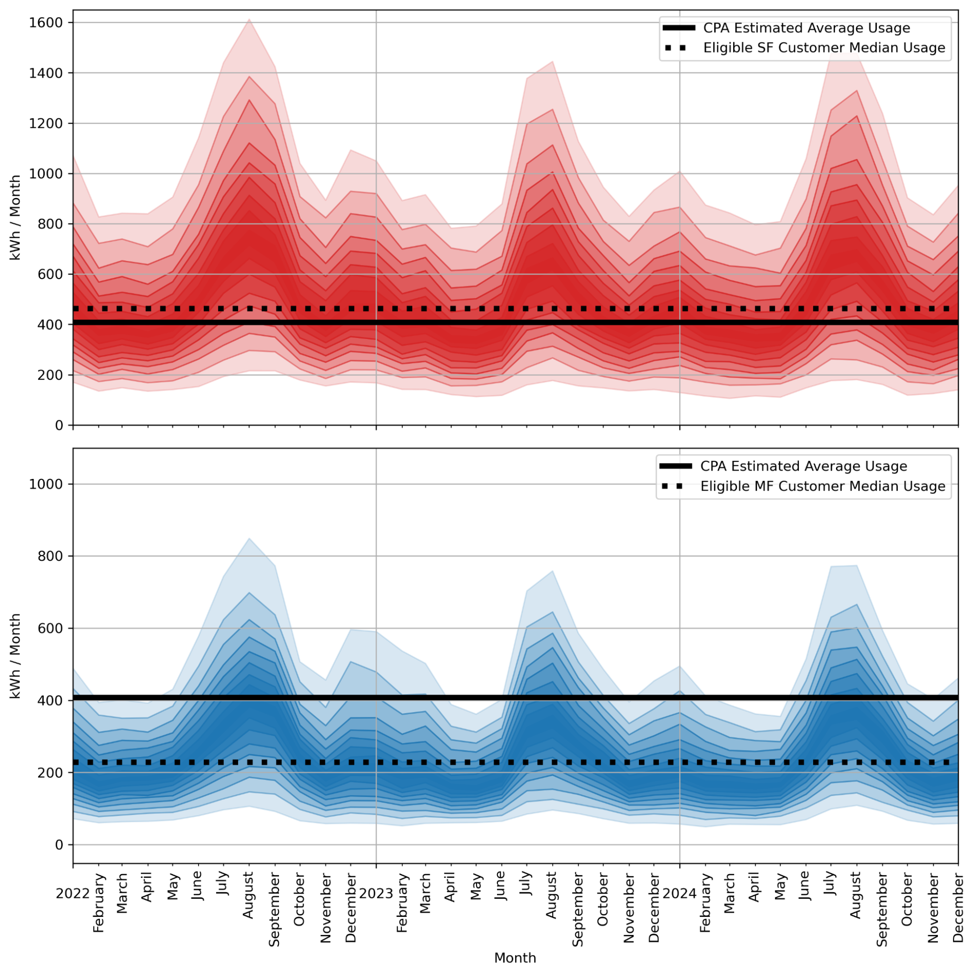
Figure 27. Fan plots illustrating the distribution (shown at 5 percentile increments) of monthly electricity usage among CSGT eligible single-family (red) and multi-family (MF) customers in our sampled usage data.
Figure 28, below, depicts the results of such a comparison that was developed using Monte-Carlo sampling procedures. In this figure, three separate colored histograms are shown. Each of these histograms depicts the distribution of total annual consumption values calculated for 10,000 unique cohorts, with each cohort consisting of 360 CSGT eligible customers - the number which corresponds to the CPA’s target enrollment cap. Each of these cohorts were repeatedly randomly selected from the sample of customer data obtained by the project team through the EDRP.
The gray histogram illustrates the range of annual usage totals that would be expected from 10,000 sampled customer cohorts for which no categorical filters were applied. Thus, the gray histogram can be thought of as representing cohorts made up of a mixture of both SF and MF customers, in different ratios. Alternatively, the red and blue histograms depict the range of annual total usage values derived from 10,000 sampled customer cohorts that were restricted to SF and MF customers only, respectively. The differences in the distribution of usage values for each of these histograms reflects the significant differences in both the average and range of monthly usage values among SF and MF customers within the BAAEC project’s eligibility area.
The solid black vertical line illustrates the total annual consumption that would be expected by multiplying the CPA’s 408 kWh / month average customer usage level by the total number of customers enrolled in the program (n = 360) and the total number of months in the program’s period of performance (12). By comparison, the broken vertical plots the total annual output in 2024 for the model’s BAAEC system based upon a scaling of another local proxy system’s actual measured hourly output.
According to this figure, we can see that the total combined usage for the CS-GT participant cohort, as derived from CPA’s quoted monthly average usage estimates, is significantly larger than the modeled BAAEC system’s output for 2024 (+34.01%). The overlap between the broken vertical line and the range of values spanned by the blue histogram, suggests that the BAAEC CS systems could likely accommodate a cohort consisting of 360 customers, providing that the majority (if not all) of those customers were multi-family property inhabitants. If a significant fraction of the 360 customers who enrolled in the CS-GT lived in single-family properties however, it is unlikely that the BAAEC systems’ output would be sufficient to fully net-out their annual electricity usage.
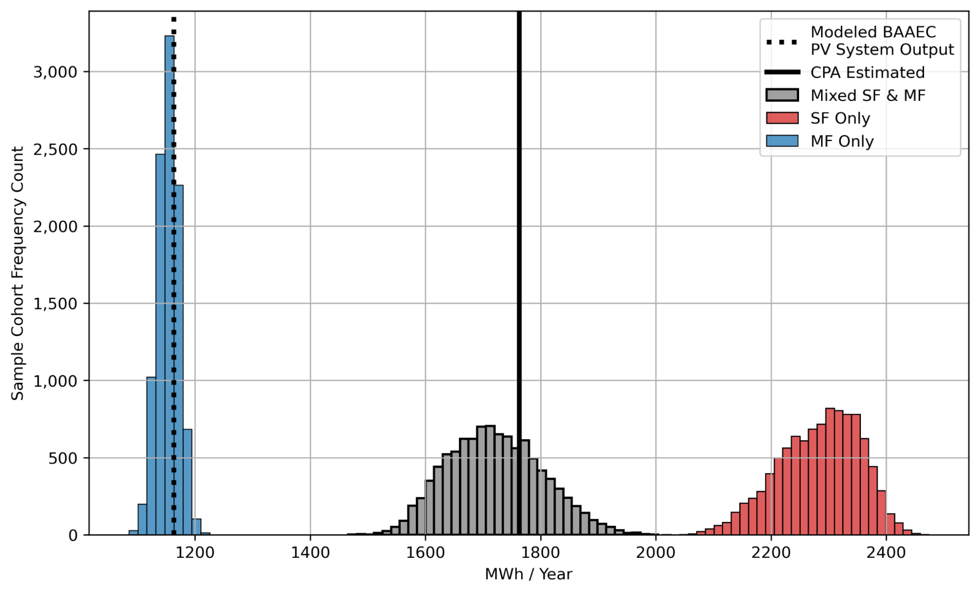
Figure 28. Monte-Carlo simulation results for the estimated total annual electricity consumption for a large number of randomly sampled customer cohorts (n = 360 customers in each cohort). Each cohort was assembled from our dataset of historical account level metered electricity usage data for CSGT eligible customers within the BAAEC geographic focus area. Results are illustrated for 10,000 randomly sampled SF-only cohorts (red), 10,000 randomly sampled MF-only cohorts (blue), and 10,000 randomly sampled Mixed SF & MF cohorts (gray). The modeled annual output of the BAAEC CS system is plotted as a broken vertical line while the CPA’s estimates for the total annual consumption of the actual participant cohort is shown as a solid vertical line.
Electricity Bill Savings
Figure 29, below, plots the range of estimated monthly electricity bill savings attributable to CSGT participation for the same set of sampled customer cohorts described previously in Figure 28. These savings values were calculated by computing 20% of each customer’s monthly bill statement amount prior to enrollment. According to this figure, the average estimated monthly bill savings ranged from $5.50 per month for the MF only cohorts to $17.56 per month for the SF only cohorts, with a value of $11.55 for the mixed SF/MF cohort group.
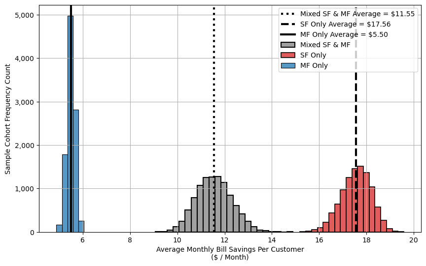
Figure 29. Estimated ranges of monthly electricity bill savings from CSGT participation for the previously sampled set of CSGT eligible customer cohorts, with the corresponding averages across each group of cohorts reported.
Avoided GHG Emissions
Figure 30 below plots the avoided GHG emissions (in CO2 equivalents) attributable to the modeled BAAEC system’s output for 2024, aggregated at an hourly (top) and monthly (bottom) interval. The avoided emissions estimates were computed by matching the hourly modeled output of the BAAEC systems to the marginal GHG emissions intensity factors for each corresponding hour obtained from data provider WattTime through the SGIP program.
There are several interesting features of note in this figure. Firstly is the large range of variability in the magnitudes of hourly avoided emissions, both on a daily and seasonal basis. This reflects the wide range of GHG emissions intensities of grid power due to variable outputs of renewable generation assets - and thus, the continued use of fast ramping fossil generation assets to cover the remaining net loads. Overall, the months with the largest magnitudes of avoided GHG emissions occur in the summer. This is generally due to the larger amounts of incident solar radiation available in these months, as well as the higher emissions intensities of grid power consumption during contemporaneous peak demand periods (e.g. those associated with cooling loads).
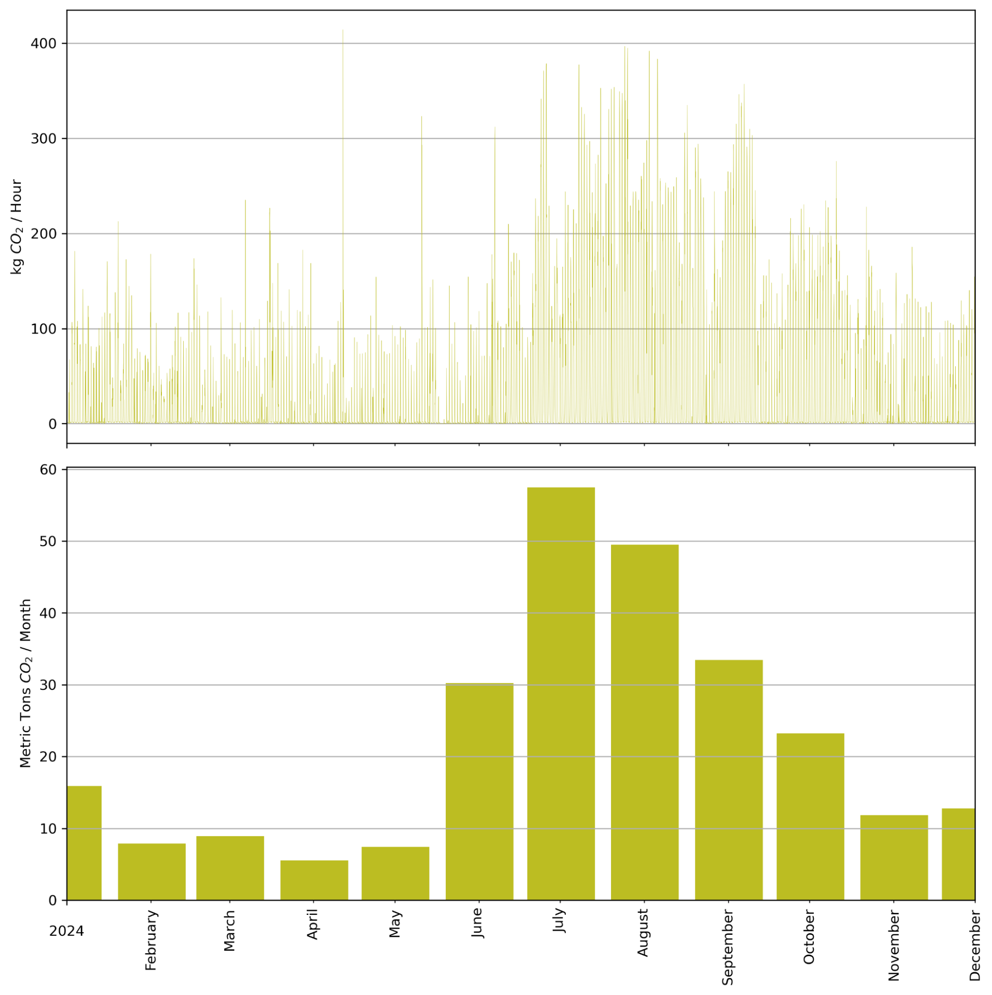
Figure 30. Avoided GHG emissions (in CO2 Equivalents) associated with the modeled output of the BAAEC Community Solar PV System for the year 2024.
The total avoided GHG emissions associated with the modeled output of the BAAEC CS sites for 2024 were computed to be 264 metric tons of avoided CO2 equivalent emissions. This equates to approximately 733 kg of avoided CO2 eq per household enrolled in the CS-GT program for that year. This value compares quite favorably with the 829 kg of avoided CO2 eq per household associated with the AH program, particularly given the relative difference in the average size of the nameplate solar PV system capacity allocations per customer between the two programs and the fact that the AH program included other load modifying measures.
Conclusions
The BAAEC project’s CS program provides an interesting counter example to its AH program as an alternative approach to deploying community scale renewable generation technologies within DACs. Under the AH program, these deployments occurred at individual customer homes, thus providing a more direct and individualized stream of benefits to community members. However, this approach effectively excluded renters and occupants of multi-tenant properties from participation. Moreover, the AH program involved significant on-site interventions associated with both the installation of various optional program measures as well as for any required site remediation work.
By contrast, the CPA’s CSGT, which the BAAEC CS program contributed to, was associated with far fewer barriers to participation. In it, customer eligibility was determined more directly by individualized need-based factors (e.g. location, household financials, billing status, etc.) as opposed to more structural characteristics (e.g. home ownership status, housing type, etc.) and the interest or availability of households to participate voluntarily. Furthermore, with the CPA’s shift to auto-enrollment, following from the BAAEC’s extensive outreach efforts in 2022 & 2023, the transaction costs associated with potential CS-GT participation were all but eliminated, save for the income verification requirement.
The principal challenges associated with the implementation of the BAAEC CS program involved locating a site which met the required design criteria of both the CPA’s CSGT pilot program and the CEC’s GFO as well as the interconnection requirements of CAISO for in-front of the meter generation assets participating in the wholesale power supply market. The intricacies of how the project team navigated these various challenges relative to the development of the BAAEC CS sites are discussed in much greater detail in the project’s Case Study reporting.
Key Findings
-
Community Solar programs can be highly successful at developing local, community scale, renewable generation assets whose outputs are sufficient to offset the full energy usage of a large number (hundreds) of customers. These benefits can either be allocated to customers on a fixed basis as a percentage of their usage, as with the CSGT’s 20% on-bill reduction, or through more sophisticated virtual net energy metering (VNEM) used in some other programs.
-
The two BAAEC CS projects were the first developed under the CPA’s Community Solar Green Tariff program. The CPA has recently reported that two new projects are slated to come online in the future; however, these will be folded into a newly revised Disadvantaged Community Green Tariff DAC-GT program.9 This is per the terms of a recent CPUC decision, which effectively terminated the CSGT.
-
Program participation can be accomplished via auto-enrollment processes that explicitly target customers who would otherwise be considered very “hard to reach” through more typical program designs. This has significant benefits from equity and justice perspectives and can provide a meaningful approach to countering criticisms to the “cost shift” argument against spending on solar program incentives.
-
This type of auto-enrollment process also presents minimal transaction costs to potential participants who, in many cases, may only be aware of their participation by virtue of the on-bill reductions which they receive as a result. Based upon our estimates, the program’s guaranteed 20% bill reduction likely equated to anywhere from $5.50 to $17.56 per customer enrolled in the program. These are potentially significant amounts for energy burdened customers, many of whom are currently, or recently have been, in arrears on their electricity bills.
-
The BAAEC CS program demonstrated that it is possible, though still quite logistically challenging, to develop multi-site aggregated systems as in-front of the meter generation projects located on dense urban sites. The two BAAEC CS sites are the first such set of aggregated generation assets which have been able to successfully interconnect to the CAISO wholesale market. Additionally, they are the first CSGT generation sites to have been developed in-basin on the rooftops of existing buildings, as opposed to ground mounted systems built on cleared land.
-
The overall GHG emissions reductions associated with the BAAEC CS systems’ modeled outputs for the year 2024 were significant, at ~264 Metric Tons of CO2 equivalent per year. The overall system’s size corresponded to roughly 1.86 kW-AC of nameplate generation capacity allocated to each household enrolled in the program.
-
Multi-family households in the BAAEC project focus area use 51% less energy than their single-family counterparts on average. This suggests that similar CS programs which target the enrollment of MF households versus SF, can provide benefits to a larger pool of customers for the same investment in generation capacity.
Discussion
In-Front of the Meter Interconnection Challenges
While not previously discussed in this EM&V analysis - there were significant obstacles associated with interconnecting the BAAEC CS program’s two aggregated generation sites to the CAISO wholesale market. The project leads at TEC had to coordinate with Pivot Energy, CPA, SCE, and CAISO to develop the power purchase agreements necessary to achieve this aggregation, to conduct required interconnection studies, and to formalize the ultimate interconnection agreements. They also had to install CAISO mandated metering, telemetry, and control hardware to facilitate wholesale market participation. Many of these steps would otherwise be considered highly unusual for a solar project of such a modest size, at least when compared to other large, utility scale, systems. These challenges were ultimately responsible for delays in the project’s completion timeline, which resulted in this analysis having to use modeled data for the system’s output during the project’s effective period of performance, as it was not yet given permission to operate.
Benefits of Auto-Enrollment
The shift from voluntary customer enrollment to an auto-enrollment scheme for the CPA’s CSGT was a very positive development. This is because it eliminates the need to undertake outreach and engagement activities necessary to educate eligible customers about the existence of the program, its eligibility requirements, and potential benefits - so as to encourage them to apply. The CPA’s ability to automatically enroll customers based upon eligibility criteria that they were already aware of, allows for the benefits of the CS system to be appropriately allocated to those in greatest need, and who likely also faced the most significant structural barriers to participating in a voluntary enrollment process.
Termination of the Community Solar Green Tariff
As a result of a May 2024 CPUC Decision, the Community Solar Green Tariff (CSGT) is now discontinued.10 According to this Decision Pacific Gas and Electric Company, San Diego Gas & Electric Company, and Southern California Edison Company (collectively, Utilities) and Community Choice Aggregators (CCAs) shall transfer all remaining un-procured capacity assigned to this tariff to the modified Disadvantaged Communities Green Tariff (DAC-GT). Procured CSGT capacity and procurement in existing active solicitations may be transferred to DAC-GT. Utilities and CCAs may transition DAC-GT-eligible customers currently enrolled in CSGT into the modified DAC-GT, unless there is no remaining capacity.
Without reviewing all of the party comments to this decision, the CPUC justified its termination of the CSGT with the fact that a dearth of implemented CS projects caused the program to fail to meet its objectives - namely: serving a specific or distinct customer group and promoting robust low income customer participation. According to the language in the Decision:
“The Commission agrees with numerous parties that the current CSGT program has failed to efficiently serve distinct customer groups. There have been no customers enrolled in CSGT since the rollout of the program, and no projects have come online. We concur with parties that the CSGT tariff’s complex requirements and customer eligibility criteria have made it challenging to attract developers and customers. When balancing the CSGT program’s lack of enrollment with the program’s overall costs, the CSGT tariff fails to efficiently serve any distinct customer group.
The Commission also agrees with parties that the CSGT tariff fails to promote robust participation among low-income customers based on the lack of enrollment by low-income customers. As the current CSGT tariff fails to meet two of the three goals of Pub. Util. Code Section 769.3(b)(1)(A), it is not necessary to determine whether the CSGT tariff minimizes duplicative offerings. Accordingly, the Commission finds that the CSGT tariff fails to meet the goals of Pub. Util. Code Section 769.3(b)(1)(A)”
Appendix A
====================================================================================================
Pre-Implementation - Electricity - Breakpoint Regression Results
====================================================================================================
No. Observations                   178311
No. Model Parameters                    4
Degrees of Freedom                 178307
Res. Sum of Squares           1.48053e+05
Total Sum of Squares          1.68978e+05
R Squared                        0.123832
Adjusted R Squared               0.123812
Converged:                           True
====================================================================================================
                    Estimate      Std Err            t        P>|t|       [0.025       0.975]
----------------------------------------------------------------------------------------------------
const               0.835857       0.0127       65.938           0.0      0.81101       0.8607
alpha1           -0.00970587     0.000845      -11.489      1.54e-30    -0.011362   -0.0080501
beta1               0.120559      0.00125       96.491             -      0.11811      0.12301
breakpoint1          19.4741       0.0604            -             -       19.356       19.593
----------------------------------------------------------------------------------------------------
These alphas (gradients of segments) are estimated from betas (change in gradient)
----------------------------------------------------------------------------------------------------
alpha2              0.110853     0.000921       120.42           0.0      0.10905      0.11266
====================================================================================================
Davies test for existence of at least 1 breakpoint: p=1.12106e-118 (e.g. p<0.05 means reject null
hypothesis of no breakpoints at 5% significance)
====================================================================================================

====================================================================================================
Post-Implementation - Electricity - Breakpoint Regression Results
====================================================================================================
No. Observations                   217376
No. Model Parameters                    4
Degrees of Freedom                 217372
Res. Sum of Squares           3.49909e+05
Total Sum of Squares          3.59608e+05
R Squared                        0.026971
Adjusted R Squared               0.026953
Converged:                           True
====================================================================================================
====================================================================================================
                    Estimate      Std Err            t        P>|t|       [0.025       0.975]
----------------------------------------------------------------------------------------------------
const                1.12677       0.0111        101.1           0.0       1.1049       1.1486
alpha1            -0.0412726     0.000604      -68.276           0.0    -0.042457    -0.040088
beta1               0.174559      0.00367       47.567             -      0.16737      0.18175
breakpoint1            27.53         0.09            -             -       27.354       27.706
----------------------------------------------------------------------------------------------------
These alphas(gradients of segments) are estimated from betas(change in gradient)
----------------------------------------------------------------------------------------------------
alpha2              0.133287      0.00362       36.824      6.4e-296      0.12619      0.14038
====================================================================================================
Davies test for existence of at least 1 breakpoint: p=0.0 (e.g. p<0.05 means reject null hypothesis
of no breakpoints at 5% significance)
====================================================================================================
Appendix B
====================================================================================================
Pre-Implementation - Gas - Breakpoint Regression Results
====================================================================================================
No. Observations                   178311
No. Model Parameters                    4
Degrees of Freedom                 178307
Res. Sum of Squares               594.518
Total Sum of Squares              618.637
R Squared                        0.038986
Adjusted R Squared               0.038965
Converged:                           True
====================================================================================================
                    Estimate      Std Err            t        P>|t|       [0.025       0.975]
----------------------------------------------------------------------------------------------------
const              0.0964678     0.000939        102.7           0.0     0.094627     0.098309
alpha1           -0.00377256     6.74e-05      -55.971           0.0   -0.0039047   -0.0036405
beta1             0.00339043     8.26e-05       41.055             -    0.0032286    0.0035523
breakpoint1          17.7233        0.135            -             -       17.459       17.988
----------------------------------------------------------------------------------------------------
These alphas (gradients of segments) are estimated from betas (change in gradient)
----------------------------------------------------------------------------------------------------
alpha2          -0.000382135     4.77e-05      -8.0082      1.17e-15  -0.00047566  -0.00028861
====================================================================================================
Davies test for existence of at least 1 breakpoint: p=5.22843e-72 (e.g. p<0.05 means reject null
hypothesis of no breakpoints at 5% significance)
====================================================================================================

====================================================================================================
Post-Implementation - Gas - Breakpoint Regression Results
====================================================================================================
No. Observations                   217376
No. Model Parameters                    4
Degrees of Freedom                 217372
Res. Sum of Squares               452.859
Total Sum of Squares              464.851
R Squared                        0.025798
Adjusted R Squared               0.025781
Converged:                           True
====================================================================================================
                    Estimate      Std Err            t        P>|t|       [0.025       0.975]
----------------------------------------------------------------------------------------------------
const              0.0605771     0.000683       88.712           0.0     0.059239     0.061915
alpha1           -0.00260532     4.66e-05      -55.947           0.0   -0.0026966    -0.002514
beta1             0.00249459     5.86e-05       42.561             -    0.0023797    0.0026095
breakpoint1          17.9892        0.127            -             -        17.74       18.238
----------------------------------------------------------------------------------------------------
These alphas(gradients of segments) are estimated from betas(change in gradient)
----------------------------------------------------------------------------------------------------
alpha2          -0.000110723     3.56e-05      -3.1109       0.00187  -0.00018048  -4.0963e-05
====================================================================================================
Davies test for existence of at least 1 breakpoint: p=0.0 (e.g. p<0.05 means reject null hypothesis
of no breakpoints at 5% significance)
====================================================================================================
-
Please see Case Study and Residential Energy Systems Report for details on delays ↩
-
California Self-Generation Incentive Program. Greenhouse Gas Emissions Signal. Accessed: August, 2025. https://content.sgipsignal.com/ ↩
-
US-EPA. Greenhouse Gas Emissions Factors Hub. Accessed: August, 2025. https://www.epa.gov/system/files/documents/2025-01/ghg-emission-factors-hub-2025.pdf ↩
-
GHG Signal provided by WattTime, per SGIP https://content.sgipsignal.com/ ↩
-
DNV GL Energy Insights. 2019 Residential Appliance Saturation Survey (RASS). California Energy Commission. July 2021. CEC-200-2021-005-ES. https://www.energy.ca.gov/data-reports/surveys/2019-residential-appliance-saturation-study ↩
-
Denholm, Paul, et al. Overgeneration from Solar Energy in California. A field guide to the duck chart. No. NREL/TP-6A20-65023. National Renewable Energy Lab.(NREL), Golden, CO (United States), 2015. https://doi.org/10.2172/1226167 ↩
-
Jin, Andrew S., and Kelly T. Sanders. “Characterizing residential sector load curves from smart meter datasets.” Applied Energy 366 (2024): 123316. https://doi.org/10.1016/j.apenergy.2024.123316 ↩
-
CPA’s CSGT Enrollment Criteria: https://www.cpuc.ca.gov/industries-and-topics/electrical-energy/demand-side-management/customer-generation/solar-in-disadvantaged-communities ↩
-
Clean Power Alliance. “Clean Power Alliance Board of Directors Approves Six Power Purchase Agreements for its Power Share Program.” Published: September 8, 2023. Accessed: November 13, 2025. ↩
-
CPUC Decision 24-05-065. DECISION MODIFYING GREEN ACCESS PROGRAM TARIFFS AND ADOPTING A COMMUNITY RENEWABLE ENERGY PROGRAM. Published: May 30, 2024. Accessed: November 13, 2024. https://docs.cpuc.ca.gov/PublishedDocs/Published/G000/M533/K188/533188781.PDF ↩